Engineering Optimization · Lecture Notes

Lecture Notes · Web Edition

Engineering Optimization

A practitioner's view of problems, solutions, and methods

Zhou Yanjie

Zhengzhou University

https://ieyjzhou.github.io https://ieyjzhou.github.io/lab ieyjzhou@zzu.edu.cn

Part Zero

Course Introduction

Engineering optimization is not a bag of algorithms — it is a way of thinking. It is the industry's “general practitioner”: read the whole system first, then decide which specialist tool to reach for.

第零篇 · 课程简介

The book’s logical framework & how its parts relate

The five parts form one spine: build the mindset, master the methodology, type real problems into a taxonomy, match them to a method system, then deploy in engineering.

Spine: Part Zero (mindset) → Part II (methodology) → Part III (problem taxonomy) → Part IV (method system) → Part V (deployment); new difficulties feed back, closing the “perceive → foundation → problem → method → apply → re-perceive” loop.

Chapter 0 · Course Introduction

Engineering optimization trains a way of thinking

全书的六篇（第零篇至第五篇）构成一条主线：先建立工程思维与问题意识（第零篇），继而打牢形式化与建模的基础（第一篇），再掌握通用方法论（第二篇），把实际问题归入问题谱系（第三篇）、匹配相应方法体系（第四篇），最后在工程中落地（第五篇）。

逻辑主线：第零篇（思维）→ 第一篇（基础）→ 第二篇（方法论）→ 第三篇（问题分型）→ 第四篇（方法体系）→ 第五篇（落地）；应用中的新难题再反哺问题与方法的演进，形成“认知→基础→问题→方法→应用→再认知”的闭环。

Chapter 0 · Course Introduction

The industry's general practitioner

Facing an unfamiliar engineering problem, you first play the “general practitioner”: understand the whole system, then decide which “specialist tool” to call in.

From complaint to triage: the EO mindset routes a problem to the fittest specialist method.

Chapter 0 · Course Introduction

How large and complex engineering problems are

A real engineering problem is never an isolated exercise: it ties together hundreds of facilities, variables and constraints that are tightly coupled — touch one and the whole system reacts.

One problem entangles facilities, routing, process, energy, inventory, cost, market and risk — always under uncertainty and change.

Chapter 0 · Course Introduction

What kinds of problems are there

Problems differ wildly; no single algorithm fits all. Read which “axes” a problem falls on, then pick the tool — exactly the GP’s way of typing a case.

From variables, goals, information, time, actors to data — six dimensions “type” a problem so the method fits.

Chapter 0 · Course Introduction

Solution methods: many, and complex

Solving methods are just as vast: one problem class often admits several technical routes, each branching into many concrete algorithms. The panel below is only a glimpse of that map.

From mathematical programming to heuristics, from robust to games, from simulation to learning — method richness mirrors problem richness.

Part I

Foundations

How we formalize a problem, why we decompose it, what “a solution” means, which methods exist, and the trade-offs that bind them together.

第一部分 · 基础

本篇逻辑框架

本篇奠定工程优化的语言基础：从“问题是什么”出发，到如何分解、何为解、有哪些方法，以及贯穿始终的权衡。

逻辑主线：问题 → 分解 → 解 → 方法 → 权衡，五章层层递进，构成全书的方法论地基。

CHAPTER 1

Problems

Before optimizing anything, we must say what a “problem” is — and why some are easy, some hard, and some impossible.

Chapter 1 · Problems

Three lenses on every problem

Every engineering optimization problem is, at heart, a question about choices: which design, plan, or control decision is best?

Decision problemA yes/no question. “Does there exist a schedule meeting every deadline?” — a single bit of information.

Optimization problemAsks for the best value or the best point — not merely whether a good one exists.

Engineering problemThe messy real-world problem — a container terminal, a power grid, a supply chain — we ultimately want to solve.

One hierarchy: an engineering problem is cast as an optimization problem; fixing a threshold turns it into a decision problem.

Chapter 1 · Problems

Decision problems & decidability

A decision problem is one whose answer is always “yes” or “no”. Every input maps to exactly one of two outputs.

A decision problem maps every input to one of two outputs (yes or no).

DecidableAn algorithm exists that always halts and returns the correct YES/NO answer. E.g. “does a DFA accept string $w$?” — run $M$ on $w$; time linear in $|w|$.

UndecidableNo such algorithm exists for all inputs. The Halting Problem is the classic example: Turing proved no algorithm decides it for every $(P,x)$.

Sudoku (“does a valid 9×9 completion exist?”) is decidable yet NP-complete in general. Decidability asks whether an algorithm exists; tractability asks how much it costs — different questions.

Chapter 1 · Problems

Sudoku: a decision problem in action

Puzzle: Wikipedia classic

Click a cell and enter 1–9, or use the pad below; press “Auto-fill answer” to reveal the full solution.

A real example: a genuine Sudoku puzzle below — try to complete it; this is exactly the optimization version, “find a valid completion”.

Question: “does a valid completion exist?” — the answer is a single yes/no bit.

Decidable: a backtracking search always halts with the correct answer.
Yet the general 9×9 Sudoku is NP-complete; generalised to arbitrary grid sizes no polynomial algorithm is known.
The same grid has an optimization version (find a valid completion) — which is why Sudoku returns to the optimization lens.
Try it: click a cell on the left to enter 1–9, or press “Auto-fill answer” to see the full solution at once — that is exactly what the optimization version seeks.

Chapter 1 · Problems

Modeling Sudoku: two integer-programming formulations

The game above is a decision/optimization instance. Below we write it as a strict integer program. Williams (2026) contrasts two ways to model Sudoku; the lesson is that the most natural variables for describing the puzzle are often not the ones that yield an effective linear model.

Formulation A — binary assignment

Introduce 729 binary variables: $x_{ijk}=1$ means “digit $k$ goes into cell $(i,j)$”. Every rule becomes a simple linear equality.

\[ \begin{aligned} &\sum_{k=1}^{9} x_{ijk}=1, &&\forall (i,j) &&\text{（每格恰一个数字）}\\ &\sum_{i=1}^{9} x_{ijk}=1, &&\forall j,k &&\text{（每列含 1…9 各一次）}\\ &\sum_{j=1}^{9} x_{ijk}=1, &&\forall i,k &&\text{（每行含 1…9 各一次）}\\ &\sum_{q=0}^{2}\sum_{r=0}^{2} x_{a+q,\,b+r,\,k}=1, &&\forall a,b\in\{1,4,7\},\ k &&\text{（每宫含 1…9 各一次）}\\ &x_{ijg_{ij}}=1, &&\text{若 }(i,j)\text{ 为已知 }g_{ij} \end{aligned} \]

Objective is $\min 0$ (any feasible solution). Many variables, but every constraint is a linear equality — trivial to solve, and easy to extend to Killer Sudoku (cage sums).

Formulation B — natural variables + big-M

More intuitive: just 81 integer variables $z_{ij}\in\{1,\dots,9\}$, the value of each cell. But “all-different within each row/column/box” must be linearised as a pairwise disjunction via big-M:

\[ \begin{aligned} &z_{s}-z_{t}\ge 1-M\,y_{st},\\ &z_{t}-z_{s}\ge 1-M(1-y_{st}),\\ &y_{st}\in\{0,1\},\quad M=9, \end{aligned} \]

For every pair $(s,t)$ sharing a row/column/box, add one auxiliary binary $y_{st}$ and two inequalities. That is 810 auxiliary binaries plus 1620 big-M inequalities — fewer variables, but an explosion of constraints. AMPL’s alldiff merely hides this machinery behind a high-level operator.

Python implementation (python-mip + the open-source CBC solver)

# Formulation A — binary assignment model
# (the givens below are the same puzzle shown in the figure)
from mip import Model, xsum, BINARY, minimize

N = 9
givens = [[6, 0, 8, 5, 0, 0, 0, 0, 0], [0, 0, 3, 6, 7, 9, 0, 0, 0], [4, 0, 0, 0, 3, 0, 0, 0, 7], [2, 0, 4, 0, 0, 0, 0, 8, 0], [0, 0, 0, 0, 9, 0, 0, 1, 0], [0, 9, 0, 0, 2, 4, 0, 0, 0], [0, 0, 0, 7, 0, 0, 8, 0, 2], [7, 0, 0, 0, 0, 5, 0, 0, 0], [0, 0, 0, 0, 0, 0, 3, 0, 0]]

m = Model(solver_name="CBC")            # open-source COIN-OR CBC
x = [[[ m.add_var(var_type=BINARY) for k in range(N) ]
       for j in range(N) ] for i in range(N) ]

# each cell gets exactly one digit
for i in range(N):
    for j in range(N):
        m += xsum(x[i][j][k] for k in range(N)) == 1
# each row / column contains each digit exactly once
for k in range(N):
    for i in range(N):
        m += xsum(x[i][j][k] for j in range(N)) == 1      # row i
    for j in range(N):
        m += xsum(x[i][j][k] for i in range(N)) == 1      # column j
# each 3x3 box contains each digit exactly once
for a in (0, 3, 6):
    for b in (0, 3, 6):
        for k in range(N):
            m += xsum(x[a+q][b+r][k] for q in range(3) for r in range(3)) == 1
# fix the given clues
for i in range(N):
    for j in range(N):
        if givens[i][j]:
            m += x[i][j][givens[i][j] - 1] == 1

m.objective = minimize(0)               # feasibility only
m.optimize()

sol = [[ next(k + 1 for k in range(N) if x[i][j][k].x >= 0.5)
         for j in range(N) ] for i in range(N) ]
print(sol)

Multiple solutions: enumerate with no-good cuts

A given puzzle may admit several legal completions. After each solution, append a “forbid this exact completion” cut and re-solve; stop when infeasible. This enumerates all solutions (below we keep the first few).

# continue after the model above
solutions = []
while len(solutions) < 6:
    m.optimize()
    if m.num_solutions == 0:
        break
    sol = [[ next(k + 1 for k in range(N) if x[i][j][k].x >= 0.5)
             for j in range(N) ] for i in range(N) ]
    solutions.append(sol)
    # forbid this exact completion (no-good cut)
    m += xsum((1 - x[i][j][k]) if sol[i][j] == k + 1 else x[i][j][k]
              for i in range(N) for j in range(N) for k in range(N)) >= 1
print("number of solutions found:", len(solutions))

Visualising multiple solutions

Left: the clues given by the puzzle. Middle and right: two distinct legal completions of that same puzzle. Amber-highlighted cells are where the two solutions differ — these degrees of freedom are exactly why multiple solutions exist.

Reference: A. Williams, “When Natural Variables Are Not Enough: Teaching Integer Programming with Sudoku,” arXiv:2606.30227v1 [math.OC], 29 Jun 2026.

Modeling takeawayFormulation A trades 729 “unnatural” variables for clean linear constraints; Formulation B keeps 81 “natural” variables but pays 1620 big-M inequalities for the all-different condition. Choosing variables is choosing the complexity of your constraints.

Chapter 1 · Problems

Two worked examples: decidable vs undecidable

Decidable — route feasibility (shortest path)Given a road network with lengths on each edge, “does a path from depot to customer of total length ≤ L exist?” Just run a shortest-path algorithm (Dijkstra); time is polynomial in the network size. Among the easiest decidable problems in OR.

Undecidable — tilings of the planeGiven a finite set of square tiles whose edges are each colored from a finite palette; when tiling, adjacent edges must match. “Can these tiles cover the whole infinite plane?” Berger (1966) proved this undecidable: the problem can encode the computation of any Turing machine, so it reduces to the Halting Problem — no algorithm decides it for every tile set. Stronger than NP-hard: no exact algorithm at all.

Decidability and tractability are different questions: the former asks whether an algorithm exists, the latter how much it costs. Route feasibility is decidable and efficient; whether a tile set can tile the infinite plane is undecidable — no algorithm at all. This is the gap between “can we model it” and “can we solve it” in engineering.

Two concrete instances (with diagrams)

Decidable · instance: route shortest-path feasibilityGiven a graph G, edge weights w(e), and a threshold L, “does a path from depot D to customer T of total length ≤ L exist?” Run Dijkstra from D to get shortest distances; if dist(T) ≤ L then yes. Time O((V+E) log V), polynomial in network size — an algorithm that always halts in finite steps with the correct answer.

Shortest path D→A→C→T = 5+4+5 = 14 ≤ L=15, exists; decided in polynomial time.

Undecidable · instance: can Wang tiles tile the infinite plane?Given a set of square tiles whose edges are colored from a finite palette (①②③④ here); when tiling, adjacent edges must match. “Can these tiles cover the whole infinite plane?” Berger (1966) proved this undecidable: it can encode the computation of any Turing machine, so it reduces to the Halting Problem — no algorithm decides it for every tile set.

Adjacent edges match by color (shown here). The question: can this extend forever? — undecidable.

Chapter 1 · Problems

P and NP in one breath

Class PThe decision problems solvable in polynomial time by a deterministic algorithm — the problems we can solve efficiently.

Class NPThe decision problems whose YES answers can be verified in polynomial time once a certificate is supplied; equivalently, solvable in polynomial time by a nondeterministic machine.

Because any solver can also verify its own answer, $\mathbf{P}\subseteq\mathbf{NP}$.
The central unsolved question of theoretical computer science: is $\mathrm{P}=\mathrm{NP}$?
Crucially, P and NP are defined only for decision problems — which is exactly why complexity theory keeps returning to the decision view.

Why this mattersHardness results (NP-hard, NP-complete) are stated for decision versions; proving the decision version hard proves the optimization version hard too.

Chapter 1 · Problems

NP-hard vs NP-complete

NP-hardA problem is NP-hard if every problem in NP reduces to it in polynomial time — “at least as hard as the hardest problem in NP.” If any NP-hard problem had a polynomial algorithm, then $\mathrm{P}=\mathrm{NP}$. An NP-hard problem need not be a decision problem, nor even lie in NP (e.g. the optimization form of TSP).

NP-completeA decision problem that is in NP and NP-hard — whose YES answer can be verified in polynomial time once a certificate is given.

Why complexity lives in the decision viewThe optimization form of TSP is NP-hard but not in NP (it is a “function-value” problem); its decision version (“is there a tour of length ≤ L?”) is NP-complete. This is exactly why complexity theory targets decision versions.

Chapter 1 · Problems · Appendix A figure (interactive)

Time complexity: polynomial vs. super-polynomial

Drag the handle at the right end of the x-axis to lengthen (or shorten) it, and watch how each function grows as n grows. Blue curves are “polynomial-time”; the red curve is “super-polynomial (exponential) time”.

← Drag the right handle to change the x-axis length (n max 1024, drag min 2) →

Polynomial (blue) Super-polynomial (red)

Function	value at n = 1024

The y-axis grows automatically with n — yet 2ⁿ climbs far faster than any polynomial: even as the axis keeps stretching, the exponential quickly fills the whole chart, which is exactly why NP-hard problems become intractable as size grows.

Chapter 1 · Problems

Optimization problems

An optimization problem asks for the best value or the best point — e.g. “among all schedules meeting every deadline, which minimizes total cost?”

Canonical form:

\[ \begin{array}{ll}\operatorname{minimize} & f(x)\\ \text{s.t.} & h_i(x)=0,\; i=1,\dots,m_1,\\ & g_j(x)\le 0,\; j=1,\dots,m_2,\\ & x\in X\subseteq\mathbb{R}^{n}.\end{array} \]

$x$: decision variables · $f$: objective · $h,g$: constraints · $X$: feasible set. An optimization problem is a decision problem equipped with a quantitative objective.

Example — 0–1 knapsack (a MIP) \[ \max\ \sum_{i\in I} p_i x_i\quad\text{s.t.}\ \sum_{i\in I} w_i x_i\le c,\; x_i\in\{0,1\}. \] The binary $x_i$ decides whether to pack item $i$; the mix of integer and continuous variables is what makes it a MIP.

We seek the point in $X$ that minimizes $f$.

Chapter 1 · Problems

Example: 0–1 knapsack (a MIP)

Instance: knapsack capacity C = 100, 8 candidate items (weight w, value p). Each may be taken at most once.

Item	w	p	p/w
1	23	92	4.00
2	31	57	1.84
3	29	49	1.69
4	44	68	1.55
5	53	60	1.13
6	38	43	1.13
7	63	67	1.06
8	85	84	0.99

Goal: choose the subset with maximum total value subject to total weight ≤ 100.

Mathematical model (mixed-integer program, MIP):

\[ \max\ \sum_{i=1}^{8} p_i x_i \quad\text{s.t.}\quad \sum_{i=1}^{8} w_i x_i \le C,\;\; x_i\in\{0,1\}. \]

# 0-1 knapsack modelled as a MIP
from mip import Model, xsum, BINARY, maximize

items = [(23,92),(31,57),(29,49),(44,68),
         (53,60),(38,43),(63,67),(85,84)]   # (weight, value)
C = 100                                       # capacity

m = Model(solver_name="CBC")                  # open-source COIN-OR CBC
x = [m.add_var(var_type=BINARY) for _ in items]

m += xsum(w * x[i] for i, (w, _) in enumerate(items)) <= C   # capacity
m.objective = maximize(xsum(p * x[i] for i, (_, p) in enumerate(items)))
m.optimize()

chosen = [i + 1 for i in range(len(items)) if x[i].x >= 0.5]
print("value", round(m.objective_value), "items", chosen)
# -> value 217, items [1, 2, 4], weight 98 / 100

The solver returns the exact optimum; the binary x_i are what make it a MIP.

MIP result: optimum value 217, pack items {1, 2, 4}, weight 98 / 100.

Chapter 1 · Problems

Same example: greedy heuristic vs MIP

Heuristic: sort by value density p/w descending, pack greedily if it fits (no backtracking).

# Greedy heuristic: best value-density first
items = [(23,92),(31,57),(29,49),(44,68),
         (53,60),(38,43),(63,67),(85,84)]
C = 100

order = sorted(range(len(items)),
               key=lambda i: items[i][1]/items[i][0],
               reverse=True)
cap, value, chosen = C, 0, []
for i in order:
    w, p = items[i]
    if cap - w >= 0:
        chosen.append(i + 1); cap -= w; value += p

print("greedy value", value, "items", chosen)
# -> greedy value 198, items [1, 2, 3], weight 83 / 100

Runs in O(n log n), but local greediness need not be globally optimal.

Method	Items	Wt	Val
MIP (CBC)	1,2,4	98	217
Greedy	1,2,3	83	198

Trade-off: the greedy gets only 198 (items 1,2,3), ≈8.8% below optimum, yet needs just O(n log n); the MIP is provably optimal but can be exponential in the worst case. This is the classic exact-vs-heuristic trade-off.

Chapter 1 · Problems

As size grows: accuracy vs time

Same set of random instances (capacity ≈ 45% of total weight), each solved by greedy and MIP (CBC). Horizontal axis is the number of items n.

Accuracy: MIP is always 100%; greedy fluctuates 80%–98% as n grows and gives no optimality guarantee.

n	Greedy val	Exact val	Acc.	Gr. t(ms)	Ex. t(ms)
9	351	366	95.9%	0.00	0.08
15	633	674	93.9%	0.00	0.38
30	1179	1191	99.0%	0.01	1.72
60	2516	2519	99.9%	0.01	7.23
100	3700	3704	99.9%	0.02	19.52
150	6244	6244	100.0%	0.03	46.19
200	7975	7978	100.0%	0.04	82.71

Appendix · reproducible

Data format (drop-in for the previous page’s code)

The greedy and MIP code on the previous pages need only a list of items and a capacity C. All 7 instances here use the JSON/Python-dict format below — expand it into items and C and both code blocks run unchanged.

# 与上一页完全兼容的数据格式（以 n=9 为例）
instance = {
    "n": 9,
    "capacity": 209,                       # 背包容量 C
    "weights": [49, 43, 30, 22, 50, 74, 89, 37, 71],   # w_i
    "profits": [36, 50, 94, 98, 74, 2, 100, 32, 85],   # p_i
}
# 展开为上一页代码所期望的形式
items = [(w, p) for w, p in zip(instance["weights"], instance["profits"])]
C = instance["capacity"]
# —— 上一页的贪心 / MIP(CBC) 代码原样可用 ——

7 test datasets (n = 9 → 200, reproducible)

Each instance is generated with a fixed random.seed: weights wᵢ and values pᵢ drawn i.i.d. from integers 1–100, capacity C = round(0.45·Σwᵢ); copy the seeds below to reproduce byte-for-byte. The 7-row results table above is computed from exactly this data.

Expand the 7 full datasets (JSON)

[
  {"n":9,"seed":41,"capacity":209,"weights":[49,43,30,22,50,74,89,37,71],"profits":[36,50,94,98,74,2,100,32,85]}
  {"n":15,"seed":1015,"capacity":435,"weights":[14,98,39,63,68,92,98,87,52,36,56,76,85,40,62],"profits":[94,80,100,2,76,96,15,53,64,53,65,43,81,83,96]}
  {"n":30,"seed":1030,"capacity":708,"weights":[8,55,99,77,21,84,25,58,66,51,97,10,58,85,19,25,1,75,19,21,2,98,39,97,99,47,55,90,37,56],"profits":[7,81,48,51,97,32,6,99,17,19,49,41,74,57,51,46,50,21,97,88,6,97,87,21,98,49,32,48,11,79]}
  {"n":60,"seed":1060,"capacity":1389,"weights":[32,26,3,5,84,18,19,12,77,21,96,38,15,46,92,67,3,43,91,19,70,50,28,16,79,29,100,5,63,19,84,49,91,39,43,48,66,86,80,39,15,21,16,99,80,89,93,10,67,46,5,74,82,42,75,65,96,94,64,62],"profits":[20,88,78,44,54,85,81,20,100,28,17,77,90,2,91,20,11,64,7,14,89,17,90,54,63,93,53,48,56,48,72,56,9,59,41,13,93,85,25,89,71,17,94,86,25,60,27,44,31,77,48,97,99,52,64,90,34,17,47,53]}
  {"n":100,"seed":1100,"capacity":2183,"weights":[4,91,29,66,98,18,6,53,17,67,25,26,79,7,72,80,90,98,52,6,63,75,31,71,5,48,51,38,62,63,17,33,21,17,61,73,38,68,66,77,54,26,73,2,92,65,92,87,14,35,34,8,22,10,63,37,94,34,28,33,27,14,56,24,45,47,32,74,69,11,79,89,26,17,69,32,11,55,71,45,63,81,1,13,14,53,92,73,70,30,67,92,98,59,67,44,20,19,86,52],"profits":[3,7,39,7,76,42,97,57,61,79,37,70,23,7,71,72,42,64,87,8,34,97,6,7,74,76,64,78,25,85,29,61,75,70,87,64,28,3,46,3,51,52,18,22,61,56,68,21,44,27,62,71,83,36,90,44,38,42,91,29,40,24,91,30,78,9,5,88,36,38,49,70,96,30,95,48,21,92,88,25,20,35,99,30,78,42,66,30,68,34,82,19,61,8,43,33,31,9,43,70]}
  {"n":150,"seed":1150,"capacity":3409,"weights":[18,54,69,13,31,3,32,2,7,62,60,69,33,26,3,66,81,82,37,59,48,57,49,92,84,49,53,77,44,17,58,66,70,17,83,36,78,22,73,3,48,55,69,20,87,38,50,83,99,8,86,24,78,77,73,94,78,22,42,46,55,59,79,66,73,49,76,42,12,7,40,65,39,6,77,9,80,35,13,59,60,63,28,40,4,67,100,79,20,98,77,57,71,59,76,27,42,12,62,13,8,46,45,14,69,20,2,39,42,78,72,96,78,43,54,74,81,20,22,83,79,68,94,19,89,82,21,16,97,22,82,22,32,36,87,38,61,30,60,7,62,88,4,24,6,62,81,20,53,91],"profits":[34,99,97,96,30,55,86,18,98,96,43,95,26,24,79,71,69,26,69,76,57,21,93,59,46,39,58,33,61,69,93,94,10,94,57,70,37,84,48,31,82,22,79,16,1,95,29,38,51,42,94,10,83,40,78,13,6,100,52,75,49,49,1,61,23,10,93,93,49,100,83,16,89,53,73,59,57,1,42,67,82,88,48,12,73,10,93,6,45,42,37,56,100,7,48,21,15,89,38,18,94,75,11,89,64,62,20,78,26,63,84,48,13,70,45,23,18,75,2,18,3,50,64,1,59,90,53,45,85,32,20,43,90,24,34,98,36,67,63,56,41,3,48,90,71,67,28,79,85,15]}
  {"n":200,"seed":1200,"capacity":4499,"weights":[40,80,41,13,97,85,83,10,26,93,33,6,63,58,18,26,79,78,32,58,2,33,70,59,67,26,1,61,82,25,97,8,56,85,23,23,25,77,43,32,98,27,49,5,62,16,75,5,87,17,51,91,62,32,42,2,92,28,49,6,54,32,49,35,8,86,75,37,19,42,39,40,49,83,73,54,30,75,72,43,11,64,99,23,35,6,26,37,91,80,74,13,41,73,26,91,74,82,18,94,69,79,17,13,32,7,55,12,94,64,76,100,8,5,99,84,20,98,25,60,21,10,93,3,8,88,81,12,5,49,5,9,71,70,71,2,100,82,90,8,36,65,81,21,25,35,47,74,87,46,3,56,10,43,79,67,79,96,39,43,58,77,12,82,33,60,46,31,16,55,12,98,43,80,12,73,53,1,60,72,18,32,74,91,4,65,68,53,17,77,75,50,91,87,93,72,82,24,73,87],"profits":[12,90,44,4,14,31,11,98,30,93,22,54,58,98,90,4,52,43,25,84,65,54,35,19,22,76,46,25,94,35,32,37,71,8,88,88,66,83,93,100,28,60,88,88,88,61,84,100,10,95,80,58,35,53,90,87,42,60,61,47,87,23,78,98,45,38,32,75,9,62,42,57,39,58,41,24,100,12,93,23,23,71,27,31,85,31,88,95,46,41,54,22,31,30,24,76,22,4,29,48,63,22,40,13,98,39,100,26,36,41,5,45,69,20,38,74,86,9,18,19,94,24,64,52,52,32,18,93,67,96,47,52,71,79,79,79,23,75,82,27,45,87,44,31,84,82,8,7,54,16,98,29,57,28,35,40,39,19,12,19,13,51,8,32,72,49,49,69,56,60,20,75,46,66,8,23,46,16,80,63,38,89,99,37,36,47,30,95,5,59,10,56,77,32,96,65,13,34,5,97]}
]

item i	weight wᵢ	value pᵢ	ratio pᵢ/wᵢ	greedy	exact
1	49	36	0.73		✓
2	43	50	1.16		✓
3	30	94	3.13	✓	✓
4	22	98	4.45	✓	✓
5	50	74	1.48	✓	✓
6	74	2	0.03		✓
7	89	100	1.12		✓
8	37	32	0.86		✓
9	71	85	1.20	✓	✓

Chapter 1 · Problems

Engineering problems

An engineering problem is a real-world problem in which we must choose the best design, plan, or control decision. Engineering optimization uses models and algorithms to make that choice.

Most are NP-hardScheduling, routing, packing, network design — no known polynomial exact algorithm. Exact methods become impractical beyond modest sizes.

Many are onlineDecisions made sequentially as new data arrive; by the time the instance is complete, the moment to decide has passed. Judged by competitive analysis.

A productive circleReal systems suggest problems → theory supplies the machinery → solutions feed back into better designs, posing new (harder) problems.

This is why the best solution we can deploy is almost never the theoretical optimal one — and why a formal model is indispensable even when we solve by heuristics or learning.

Chapter 1 · Problems

An engineering problem is more than optimization or decision

The real problem on an engineer's desk carries far more than the mathematical lenses capture. The model is a powerful tool for a messier whole, not the whole itself.

Contested objectives: “best” is rarely given; stakeholders pull it apart.
Human & organizational context: contracts, regulations, safety codes never appear as equations.
Implicit constraints: physical law, unwritten rules, hard-won experience.

Uncertainty & dynamics: many problems are online; the world moves while we solve.
Messy data: sparse, noisy, biased, fast.
Risk, safety, ethics: a point feasible and “optimal” on paper can be unsafe or unfair.

The mature engineer solves the model and then asks what the model left out.

Chapter 1 · Problems

Online vs offline problems

Offline (batch) problemFully specified before any decision: all data, parameters, the complete instance are known, so a solution can be computed at leisure.

Online problemData revealed step by step; each decision must be made before later data arrive, and earlier decisions usually cannot be undone.

How to judge an online algorithmBy competitive analysis: compare its cost with the optimum of a clairvoyant offline instance that would have known everything in advance. E.g. orders arrive over time, a machine fails unexpectedly — by the time data are complete, the moment to decide has passed.

Chapter 1 · Problems

One hierarchy: engineering → optimization → decision

The three classes nest by containment; the outer set is broadest.

Optimization and decision are polynomially equivalent:

Lemma — optimization reduces to decisionIf an optimization problem is solvable in time $T$, its decision version is solvable in time proportional to $T$: fix a threshold $B$, solve the optimization problem, compare the optimum with $B$.

Each step refines the previous; the decision version is the simplest — and complexity theory lives there.

Chapter 1 · Problems

Recovering the optimum by binary search

The converse also holds: with a decision oracle — “is there a feasible $x$ with $f(x)\le B$?” — we recover the optimum by binary searching $B$ over an interval. This is the converse of the lemma; together they prove decision and optimization are polynomially equivalent.

If the objective is integer-valued in a known interval $[L,U]$, about $\lceil\log_2(U-L)\rceil$ queries pin down the optimum exactly.

Chapter 1 · Problems

Why mathematical models?

Before choosing a method, answer the decisive question: can this problem be cast as a mathematical model?

Communication. A formulation is a universal language that removes ambiguity about what is optimized and under what conditions.
Baseline for evaluation. The model optimum is the benchmark every heuristic, learning method, or simulation must beat.
Education. Multiple formulations of one problem become a teaching asset — training adaptable, critical thinking.
Scaling with learning. ML exploits structural features to soften solver limits, opening MILP to larger, realistic problems.

When formulation failsObjective contested, constraints unwritable, system poorly understood, or data too fast/messy → fall back on learning, heuristics, and simulation.

Chapter 1 · Problems

Modelable vs. non-modelable

Modelable → mathematical methodsComponents: objective $f(x)$, decision variables $x$, constraints. Solvers: Gurobi, CPLEX (commercial); GLPK, CLP, SCIP, CBC (open-source); BARON (global NLP).

Heuristics & metaheuristics (GA, PSO, SA): good solutions without a closed-form model.

Machine learning: learns the mapping from features to decisions.

Simulation: imitate the real process, choose the best in silico.

The boundary is not absolute: a problem only partially modeled today may be fully modeled tomorrow. The honest first question — “can we write it down?” — dictates the entire toolkit that follows.

Chapter 1 · Problems · §1.5.4

MIP is NP-hard, linear programming is in P

MIP — NP-hardInteger/binary restrictions make the general mixed-integer program NP-hard (Karp, 1972). No polynomial exact algorithm is known; solvers fall back on branch-and-bound / branch-and-cut / heuristics at scale.

LP — in POnly continuous variables and linear constraints. Karmarkar (1984) gave an interior-point method solving LP in polynomial time → $\mathrm{LP}\in\mathrm{P}$. (Simplex is fast in practice but exponential worst-case.)

But complexity is a growth rateEven an LP can have tens of millions of variables; such instances still need days or weeks (Klotz & Newman, 2013). And linear programming cannot solve large NP-complete problems in polynomial time (Hofman, 2006): the relaxation is fast, but it does not deliver an exact integer solution.

That boundary — provable exact method exists (LP) vs. provably does not (MIP) — is why the rest of the book invests in decomposition, learning, and heuristics for the integer case.

Chapter 1 · Problems · hands-on

Container relocation: an interactive NP-hard puzzle

Retrieve the boxes in priority order 1,2,3,… . If the target box is buried, you must first relocate the boxes on top to other stacks — each relocation counts as one “reshuffle”. The goal is to clear all boxes with the fewest relocations.

Rules: ① Stacks grow bottom→top with a max-height cap; you may only move the top box of a stack onto the top of another (no placing on a full stack). ② Retrieve in the fixed order 1→2→3… (always the current global-minimum priority): if the target is already on top, take it directly (no relocation); if buried, first move every box above it to other stacks, +1 relocation each. ③ Score = number of relocations (lower is better); move distance / time are also tracked from the yard parameters. ④ Variants: Restricted (only blockers of the current target may move) / Unrestricted (any top box may be moved early to optimize ahead).

How to play: press and drag the topmost box onto another stack to relocate it; to retrieve, drag it onto the “Outlet” on the right (only allowed when it is the current global minimum).

🚚

Outlet

Level:

Rule:

Yard parameters (configurable)

Bay spacing (m): Handling time (s): Transit per m (s/m):

Your moves (step by step)

Optimal solution

Click “Compute optimal” to see the minimum relocations and the plan.

Your score

Moves0

Distance0 m

Time0 s

Optimal baseline

Min moves—

Min dist—

Min time—

Chapter 1 · Problems · digression

The long road to NP-hardness: container relocation

2006 · Kim & HongFirst defined the problem and gave a branch-and-bound algorithm that is guaranteed optimal. Exact, yet its running time grows steeply with size.

2012 · Caserta et al.Gave a mathematical formulation and proved the problem NP-hard. The formal hardness result arrived six years after engineers began studying it.

Solve first, theorize laterThe usual engineering order: deliver a working method (heuristic, branch-and-bound, learned policy) first, and only afterwards ask whether a formal hardness result explains why it was hard. The NP-hard label is retrospective confirmation, not a prerequisite; the absence of a proof never stops engineering.

References

CHAPTER 2

Problem Decomposition

Big problems rarely solve as one block. We split, solve locally, and coordinate.

Chapter 2 · Decomposition

Why decompose?

Scale: a 2,000-vehicle routing problem is intractable as one monolith.
Structure: loosely coupled sub-systems interact only through a few shared quantities.
Parallelism: independent sub-problems solve concurrently.
Expertise: different teams own different sub-problems.

The catchDecomposition is free to draw but costly to coordinate — the cut must land where coupling is weakest.

Chapter 2 · Decomposition

Divide-and-conquer & 分而治之

Western: divide-and-conquerRecursively split a problem into same-kind sub-problems, solve, then combine — with the recombination cost made explicit (merge sort $O(n\log n)$, quicksort degrades to $O(n^2)$).

Chinese: 分而治之“Divide in order to govern.” Emphasis on when to divide and how the parts stay whole — 分与合 as an oscillating movement (分久必合，合久必分).

Split → solve → combine. The combine step is where cost (and risk) lives.

Chapter 2 · Decomposition

Real engineering cases

Construction & demolition (C&D) logistics: spatial + stage decomposition (collect → transfer → sort → dispose); the recycling plant is the bottleneck → tightly coupled coordinator.
Large construction program scheduling: decompose by agent / zone; shared tower cranes, hoistways, site roads create tight coupling → a program-level scheduler coordinates.
Wafer-fab scheduling: recursive / hierarchical decomposition + re-entrant flows; tool groups are the bottleneck → a fab-level dispatcher coordinates. Echoes the Benders / Dantzig–Wolfe methods of Part IV.

Chapter 2 · Decomposition

A decomposition example: city delivery (Zhengzhou)

Cut the monolithic “same-day city delivery” along two axes: space and time window. We use central Zhengzhou as the example.

By space: split Zhengzhou into 8 operating zones, ~250 orders each.
By time window: each zone splits into morning / afternoon batches.
Solve in parallel: 16 sub-problems each run a routing solver; hours shrink to minutes.
Coordinate: cross-district orders and the shared fleet are handled by an upper coordinator.

Central Zhengzhou: heatmap = order density, white dashed lines = 8 operating zones; the Yellow River lies to the north, with the Jingguang / Longhai railways crossing.

Chapter 2 · Decomposition

A numerical decomposition example

Take “warehouse location – delivery”: the master decides which warehouses to open; the sub-problem routes deliveries given those warehouses. One iteration coordinates them.

The master fixes “which warehouses”, the sub-problem returns cost plus a feasibility cut; the master updates its decision.

Iteration 0The master guesses “open A only”. The sub-problem finds B-zone orders miss their deadlines → infeasible, and returns a cut: another warehouse must open.

Iteration 1The master adds the cut and guesses “open A and B”. The sub-problem finds cost 80 and all feasible → coordination done, a global feasible solution is obtained.

Chapter 2 · Decomposition

Five recurring cuts of decomposition

Every problem differs, yet the same few cuts recur. Recognising them lets you reach for the right coordination mechanism later.

By decision agent — split among independent actors (bilevel / Stackelberg).
By time horizon — planning / scheduling / control at different scales.
By spatial region — weakly coupled subsystems (berths, yards, vehicles).
By objective — scalarise then reconcile (goal programming).
Hierarchical / recursive — decompose again until each leaf is solvable (Benders, Dantzig–Wolfe).

One hard whole can be split along five recurring dimensions; the right cut depends on the problem's structure.

Chapter 2 · Decomposition

How to choose the cut: draw a coupling graph

The first step of decomposition is not “how to cut” but “where to cut”. Draw the system as a graph: nodes are sub-systems, edges are their dependencies and data exchanges, and an edge’s “thickness” is its coupling strength.

Cut at weak coupling: the cut should cross the thinnest edges — fewer severed dependencies means a lighter load on the coordinator.
Shorter cut, cheaper coordination: a longer cut means more variables cross the boundary, so coordination costs more.
Balance the cut: one side too large is still intractable; trade off “independently solvable” against “weakest coupling”.

Keep strong couplings on the same side (A–B, C–D); let only the thin weak edges become the coordination channel.

Chapter 2 · Decomposition

Two coordination regimes

Loosely coupled: a single boundary exchange. Tightly coupled: a coordinator iterates parameters and solutions with every sub-problem.

Chapter 2 · Decomposition

Two coordination regimes: loose vs tight

Splitting creates coupling constraints — the shared variables that tie sub-problems together. A valid solution respects not only its own constraints but also the coupling.

RuleLoosely coupled sub-problems exchange a few boundary values; tightly coupled ones (a single bottleneck resource) need a coordinator — a master problem or an iterative scheme — to drive them to a globally consistent solution.

Chapter 2 · Decomposition

Container terminal: four weakly-coupled sub-problems

A container terminal must, at minimum, allocate berths, schedule quay cranes, stack the yard, and route vehicles — each with its own variables, constraints, and best method.

The whole is never solved at once; it is solved as a federation of tractable parts. The shared quantities are negotiated until consistent.

Chapter 2 · Decomposition

A counterexample: a wrong cut is worse than none

Recall the warning from s-c2a: decomposition is free to draw but costly to coordinate. If the cut lands on the strongest coupling, the coordinator becomes a throughput bottleneck; iterations explode and the communication / recomputation cost overwhelms whatever solve time the decomposition saved.

Wrong cut: split a pair of strongly-coupled sub-systems that should sit together → every interaction between them must now round-trip through the coordinator.
Consequence: the coordinator is both slow and a single point of failure; the whole becomes slower and more fragile than the monolith.
Remedy: first draw the coupling graph (s-c2i) and let the cut cross the weakest edges; if no good cut exists, prefer not decomposing at all to cutting badly.

Splitting a strongly-coupled pair forces every exchange between them to first pass through the coordinator.

Chapter 2 · Decomposition

The cost & risk of decomposition

Consistency: each sub-problem optimal ≠ globally optimal; split local solutions fight at the boundaries.
Coordination overhead: under tight coupling iterations can explode; communication and recomputation cost exceed the gains.
Lost global view: cross-cutting trade-offs (e.g. safety vs cost) become invisible; locally pretty, globally poor.
Wrong cut: cutting where coupling is strongest makes the coordinator the bottleneck — worse than not decomposing.
Slow convergence: iteration may converge slowly; in practice we often stop when “good enough” and accept sub-optimality.

In one lineDecomposition is a means, not an end — a wrong cut is worse than none.

Chapter 2 · Decomposition

Does decomposition give the true optimum?

Not necessarily. It depends on whether the coordinator can prove convergence.

Exact decompositionBenders / Dantzig–Wolfe: master and sub-problems exchange cuts and bounds repeatedly; once converged it is provable — the decomposed solution equals the whole’s global optimum. Decomposition is merely an algorithmic device; it does not change the answer.

Heuristic decompositionGreedy splits, fixed iteration counts, or “stop when good enough” ADMM: what you get is a feasible / near-optimal solution, with no optimality certificate. It is cheap and fast, but you should know exactly what guarantee you gave up.

One-line testIf the coordinator can prove convergence (cuts converge / dual bound closes) → decomposed = global optimum; otherwise it is only feasible or near-optimal. The warehouse-location example in this chapter is the former; the city-delivery “16 sub-problems solved separately” is often the latter if never coordinated.

Same word “decomposition”, very different certainty of the answer.

Chapter 2 · Decomposition

Chapter 2 takeaways

Big problems lean on decomposition; decomposition leans on the cut; the cut must land where coupling is weakest.
Western “divide-and-conquer” prices the combine step explicitly; Chinese “分而治之” stresses the oscillation of divide-and-unite and the whole.
Loosely coupled: one boundary exchange. Tightly coupled: a coordinator iterates with the sub-problems.
Decomposition is no free lunch: consistency, overhead, and global visibility all carry a price.
The rest of the book (Benders / Dantzig–Wolfe / heuristics) is the concrete answer to “how to cut, how to coordinate”.

Chapter 2 · Decomposition

Case: a container terminal as four sub-problems

Berth allocation: where each arriving vessel moors.
Quay-crane scheduling: which bays each crane serves.
Yard planning: where import/export boxes are stacked.
Horizontal transport: AGVs/trucks move boxes between quay and yard.

The cut lands where coupling is weakest: berth/yard split independently, quay–yard–transport coordinate tightly.

Chapter 2 · Decomposition

Case: C&D waste logistics decomposition

By space: collection points, transfer stations, sorting centres and disposal sites sit at different locations.
By stage: collect → transfer → sort → dispose is a serial pipeline.
Bottleneck: the recycling plant has limited throughput → it becomes the tightly-coupled coordinator.

Cut the whole chain along space and stage; the recycling plant's throughput makes it the global bottleneck.

CHAPTER 3

Solution

“A solution” is not one thing. Feasible, local, global, near-optimal — each means something precise.

Chapter 3 · Solution

Feasible · Local · Global

Feasible set (Table 3.1 notation): \[ X=\{\,x\in\mathbb{R}^{n}: h_i(x)=0\ (i=1,\dots,m),\; g_j(x)\le 0\ (j=1,\dots,p)\,\}. \]

Feasible solution$\hat{x}\in X$: satisfies every constraint.

Local optimum (minimization)$\exists\,\varepsilon>0:\ f(x^\star)\le f(x),\ \forall x\in X\cap B_\varepsilon(x^\star)$.

Global optimum (minimization)$f(x^\star)\le f(x),\ \forall x\in X$, i.e. $x^\star\in\arg\min_{x\in X}f(x)$.

Default: minimization. For maximization reverse the inequalities and swap min↔max.

The grey shade is the feasible set X; the red dot is a local optimum (lowest in its neighbourhood, yet not global), the blue dot the global optimum. The cross outside marks an infeasible point.

Chapter 3 · Solution

Near-optimal solution

Near-optimal (ε-optimal), minimization \[ f(\tilde{x})\le f(x^\star)+\varepsilon,\quad\text{i.e. }\tilde{x}\in\{\,x\in X: f(x)\le f(x^\star)+\varepsilon\,\}. \]

In engineering we rarely prove the global optimum; we usually settle for a provably near-optimal one — and that certificate (a bound on the gap) is often what shipping decisions actually require.

NoteMaximization: $f(\tilde{x})\ge f(x^\star)-\varepsilon$.

Below the red dashed line (light-red band) lies the ε-near-optimal set: every point there has objective no worse than the global optimum plus ε. In practice we often accept such an x~ and ship the “gap ≤ ε” certificate.

Chapter 3 · Solution

Non-convex landscapes: 2-D contours vs 3-D relief

The same non-convex landscape: top-down it is nested contours, side-on it is the real relief. The 3-D view makes “deeper global basin, shallower local basin, the ridge, the flat region” obvious at a glance — exactly the features that trap, stall, or zig-zag gradient search.

Top-down contours: blue basin = global, red = local, warm ridge, yellow flat region; green dashed = gradient path.

Drag the surface to rotate; blue = global optimum (2.0,−1.5), red = local (−1.8,1.8), warm ridge across the middle.

Chapter 3 · Solution

A numeric mini-example: local ≠ global

Consider the 1-D objective $f(x)=\sin x$ on $x\in[0,4\pi]$, minimized.

Local optimum: starting at $x=1$ and walking downhill, you stop at $x=\tfrac{3\pi}{2}\approx4.71$, $f=-1$.
Global optimum: the same function also hits $-1$ at $x=\tfrac{7\pi}{2}\approx10.99$ — here they tie, but in higher dimensions local points are usually worse.
Lesson: gradient methods are “near-sighted” and easily stop at the first valley; global search needs multiple starts, randomness, or a global method.

Descent from the left stops at the first (shallower) valley — unaware of the deeper global one further right.

Chapter 3 · Solution

Why convexity matters: convex ⇒ local = global

The previous section showed: in non-convex landscapes, gradient methods stop at the first valley. Convexity is the watershed — it makes “local optimum” and “global optimum” the very same thing.

Convex problemThe feasible set $X$ is convex and the objective $f$ is convex (a downward bowl). Any local optimum is automatically global — no fear of “did we miss a lower valley”.

Non-convex problemPits and ridges exist, so local ≠ global optimum. This is one root of “LP ∈ P but MIP is NP-hard”: linear programming is convex, mixed-integer programming is not.

In a convex landscape you always slide to the one valley; in a non-convex one, which valley you reach depends on where you start.

Chapter 3 · Solution

Convex sets & convex functions: the two building blocks

The previous section claimed "convex ⇒ local = global". Convexity rests on two independent notions, each needing a formal definition.

Convex set XAny segment between two points stays inside: $\forall x_1,x_2\in X,\ \forall\lambda\in[0,1],\ \lambda x_1+(1-\lambda)x_2\in X$.

Convex function fAny chord lies above the graph: $\forall x_1,x_2,\ \forall\lambda\in[0,1],\ f(\lambda x_1+(1-\lambda)x_2)\le \lambda f(x_1)+(1-\lambda)f(x_2)$.

A "convex function" opens upward (a bowl), its chords sitting above the graph. A linear function is both convex and concave — the other face of why LP is easy and MIP hard.

Chapter 3 · Solution

From local toward global

Since gradient methods are near-sighted, finding the global optimum means widening the view. The common strategies boil down to two ideas: try several starts, or occasionally allow a step uphill.

Multi-start / random restart: run gradient descent from many random starts, keep the best valley. Simple, parallel-friendly, but no guarantee of the global. E.g. in production scheduling, run local improvement from several initial schedules and keep the best.
Simulated annealing: accept “temporarily worse” steps with some probability, escaping local valleys as temperature cools; the cooling schedule trades exploration against exploitation. E.g. in VLSI placement, “heated” acceptance of worse layouts avoids getting stuck in a cramped local arrangement.
Evolutionary / swarm algorithms: keep a “population” and search broadly via selection, crossover, mutation; good for black-box, non-convex, high-dimensional problems. E.g. vehicle routing (VRP) often uses genetic algorithms for broad search over fleet assignments, yielding near-optimal tours.
Exact methods as backstop: if the problem is convex or a small MIP, branch-and-bound / Benders can prove the global optimum — no need for the “lucky dip” strategies above. E.g. structured MIPs like airline crew scheduling are solved by solvers that return an optimal roster with a gap certificate.

RememberA gradient method guarantees a local optimum; a global one usually needs multi-start, randomness, or an exact method — which is exactly what Chapter 4 (“Methods”) unpacks.

Chapter 3 · Solution

Optimality conditions: what makes a point “optimal”

We have defined "local" and "global". But given a candidate point, how do we tell whether it is optimal? The answer is a checkable set of conditions.

Unconstrained (1st-order necessary)$\nabla f(x^\star)=0$: at an optimum there is no downhill direction.

Constrained (KKT)For $\min f(x)$ s.t. $g_j(x)\le 0,\ h_i(x)=0$, an optimum satisfies: stationarity, primal feasibility, dual feasibility, complementary slackness. The "checklist" for a candidate.

Key insightFor a convex problem, the KKT conditions are not only necessary but also sufficient — any point satisfying them is optimal. This is the formal root of "convex ⇒ local = global", and why solvers can issue an optimality certificate.

Chapter 3 · Solution

Try it: drag the ball, watch which valley it rolls into

The curve below is the same multimodal function $f(x)$ used in the simulated-annealing demo (page 53), for $x\in[0,4\pi]$, with several local minima and one global minimum. Drag the ball anywhere; on release it “rolls downhill” to the nearest valley floor. Try several starts and see whether it always finds the true global minimum.

Release to roll downhill; different start, different valley — the tangible demo of “local ≠ global”.

Chapter 3 · Solution

Try it: multi-start & simulated annealing

The curve below has several local minima, with the deepest global minimum near x≈9. Click "Run multi-start" to descend from many random starts; click "Run simulated annealing" to allow occasional uphill jumps — the ball "heats up" and hops out of shallow valleys (with a jump arc), and see whether it finally lands in the deeper global one.

Multi-start marks every landing point (orange); the lowest is blue (global). The simulated-annealing ball "heats up" to escape the shallow valley and tends toward the deeper global one.

speed

Chapter 3 · Solution

Notation & the feasible set

Before any optimization problem can be solved we need a shared vocabulary.

Symbol	Meaning
$x\in\mathbb{R}^n$	vector of decision variables
$f(x)$	objective to minimise / maximise
$h_i(x)=0$	equality constraints
$g_j(x)\le 0$	inequality constraints
$X$	feasible set (domain of x)
$x^\star$	an optimal solution

The feasible set collects every point that satisfies all constraints:

\[ X = \{\, x\in\mathbb{R}^n : h_i(x)=0,\; g_j(x)\le 0 \,\} \]

Chapter 3 · Solution

Why proving optimality is hard in practice

The mechanisms for certifying optimality — KKT for smooth convex problems, bounds and the optimality gap for discrete ones — all assume the problem is fixed, known, and cheap to evaluate. Real engineering violates all three at once:

Non-convex, rough landscapes — many local minima, plateaus, ridges; no KKT certificate, maybe no tractable relaxation.
NP-hardness at scale — scheduling, routing, packing grow combinatorially; certifying optimality (gap = 0) is infeasible beyond modest size.
Online, shifting data — by the time you finish solving, the problem you solved is no longer the one you face.
Model & measurement error — the true objective is only a proxy $f(x)$; noisy or biased data can make a "proven" optimum far from the best real decision.
Uncertainty & risk — a point optimal in expectation can be catastrophic in the worst case.
Time, data & compute budgets — the decision moment has a deadline; waiting for a certificate is itself a cost.

UpshotIn practice we almost never determine the optimum. We bound it (the gap), settle for near-optimal or heuristic, and re-solve as new information arrives.

Chapter 3 · Solution

Best solution in practice: the toolbox

Two structural facts force us to aim for the best solution in practice: most engineering optimization problems are NP-hard, and the data usually arrives too late to wait for the optimum. We obtain it through a toolbox:

Heuristics & metaheuristicsGA, simulated annealing, tabu search, ACO — strong feasible solutions in seconds; no optimality guarantee.

MatheuristicsEmbed an exact solver inside a metaheuristic: harvest both quality and speed.

Approximation algorithmsPolynomial time with a provable worst-case bound (approximation ratio).

Rolling-horizonSolve a limited window now, commit early decisions, re-solve the next window as data arrives.

Learning-based & reactivePredict promising regions or good initial solutions; handle surprises as they arrive.

RuleSet a tolerance, run until the deadline or gap target, accept the best feasible solution on hand.

Chapter 3 · Solution

Case: online meal-delivery (no offline optimum)

Orders arrive over time: at time t the dispatcher only knows orders received so far.
The offline optimum needs foreknowledge of the future — impossible in practice.
So engineering settles for an online near-optimum with a provable competitive ratio.

The offline optimum needs all orders; future orders have not arrived yet, so only online decisions are possible.

Chapter 3 · Solution

Case: the optimality-gap certificate

Branch-and-bound keeps two bounds: the upper (best found) and the lower (best possible remaining).
Gap = upper − lower; gap 0 proves the global optimum.
What shipping needs is the certificate, not endless refinement.

When the upper (red) and lower (green) bounds meet, the gap vanishes and global optimality is proven — the certificate shipping needs.

Chapter 3 · Solution

The lifecycle of a solution

A solution travels from “problem” to “accepted” along a self-correcting pipeline: formulate, solve, obtain a candidate, test optimality; accept if optimal, otherwise accept as near-optimal or refine.

“Optimal?” is the diverter: yes issues a certificate, no accepts near-optimal or loops back. Most engineering problems stop at “near-optimal”.

Chapter 3 · Solution

Optimal in theory vs best in practice

Problems like meal-delivery scheduling do have an optimal solution in theory, but orders keep arriving (online). Waiting for every order before optimizing means the delivery windows have long expired — the dispatcher ships the “best solution available now”.

The gap between the “optimal” and the “best” solution is not a failure of methods but an inevitable cost of real-time engineering.

CHAPTER 4

Methods

Exact, heuristic, or approximate — each earns its place under different constraints.

Chapter 4 · Methods

Methods for optimization theory

Method	When it fits	Strength	Weakness
Exact (BB, BC, DP, Benders, D-W)	Faithful model, LP or small/structured MIP, need proof	Provable optimum; optimality gap certificate; mature solvers	Large MIP can explode; needs exact closed-form model
Heuristics & metaheuristics	NP-hard, high-dim, too slow for exact	Fast, flexible, handles black-box / non-convex	No optimality guarantee; result varies with run & tuning
Approximation algorithms	Need polynomial time with a bound	Polynomial time; provable worst-case bound	Bound may be loose; not all problems admit one
Learning-based (neural / RL)	Data-rich, incomplete model, online / high-dim patterns	Fast inference; captures complex patterns; end-to-end	Needs data; sim-to-real gap; less interpretable

Chapter 4 · Methods

Methods for real engineering problems

Method	Role	Trade-off
Modelling & abstraction	Coarse-to-fine simplification	Fidelity vs. tractability
Simulation-based	Evaluate, not optimize	Expensive; no gradient
Learning from data	Surrogate / policy	Needs data; sim-to-real gap
Multiple & robust choices	Hedge uncertainty	Conservative; harder model
Human-in-the-loop	Validate & revise	Slow; captures modelling errors

Chapter 4 · Methods

How to choose a method: a checklist

Small problem, faithful model → use an exact method (MILP solver, branch-and-bound). Pick it when you need an optimality certificate.
NP-hard, large, need speed → use heuristics / metaheuristics (GA, tabu, simulated annealing). Accept “good but not guaranteed optimal”.
Need a worst-case guarantee and polynomial time → use an approximation algorithm, and watch the ratio.
Inaccurate model / missing data / online → use simulation, learning, human-in-the-loop to fill the model's gaps.

Rule of thumbFirst ask “how big is this, and how certain must the answer be?” — the answer usually points straight at the method, not the other way around.

Chapter 4 · Methods

Inside exact methods: how branch-and-bound searches

An exact method does not “try every solution” — it searches systematically and prunes by bounds. For a mixed-integer program, branch-and-bound does three things:

Branch: relax integrality, solve the LP relaxation; if the solution is still fractional, split on some variable into two branches (≤k and ≥k+1).
Bound: at each node the LP-relaxation value gives a lower bound on that subtree’s best.
Prune: if a node’s lower bound is already worse than the best known integer solution (the upper bound), the whole subtree is skipped — exactly why it beats brute force.

The red dashed node: its bound is already worse than the known integer upper bound, so the whole branch is pruned.

Chapter 4 · Methods

Case: branch-and-bound for the 0-1 knapsack

Problem

A relief truck has capacity 15 (weight units) and five candidate supply boxes A–E, each with a weight and a value. Choose which to load to maximize total value without exceeding capacity.

Model

$ \max \sum_j v_j x_j \quad\text{s.t.}\quad \sum_j w_j x_j \le W,\; x_j\in\{0,1\} $

Data: A(2,40) B(3,50) C(4,65) D(5,70) E(9,110), capacity W=15.

Result

Optimal load A,B,C,D: total value 225, using 14 of 15. Branch-and-bound expanded only 11 nodes (vs 32 by brute force).

Python implementation

# Branch-and-bound for the 0-1 knapsack
items = [('A',2,40),('B',3,50),('C',4,65),('D',5,70),('E',9,110)]
W = 15
names=[t[0] for t in items]; w=[t[1] for t in items]; v=[t[2] for t in items]
n = len(items)
best = {'val': -1, 'take': None}
nodes = 0

def bound(i, cw, cv):                 # greedy upper bound on remaining items
    bw, bv = cw, cv
    for j in range(i, n):
        if bw + w[j] <= W:
            bw += w[j]; bv += v[j]
        else:
            bv += v[j] * (W - bw) / w[j]; break
    return bv

def bb(i, cw, cv, taken):
    global nodes
    nodes += 1
    if i == n:
        if cv > best['val']:
            best['val'] = cv; best['take'] = taken[:]
        return
    if bound(i, cw, cv) <= best['val']:
        return                         # prune: cannot beat incumbent
    if cw + w[i] <= W:                # branch: take item i
        taken.append(i); bb(i+1, cw+w[i], cv+v[i], taken); taken.pop()
    bb(i+1, cw, cv, taken)            # branch: skip item i

bb(0, 0, 0, [])
print('optimal value :', best['val'])
print('selected      :', [names[k] for k in best['take']])
print('nodes explored:', nodes)

Chapter 4 · Methods

A glance at metaheuristics: GA & simulated annealing

When the problem is NP-hard, non-convex, or black-box, and “a good solution is enough”, metaheuristics use controlled randomness to search broadly, trading the optimality guarantee for speed.

Genetic algorithm (GA)Keeps a population of solutions: select the fitter ones, crossover pairs to breed offspring, then mutate to inject diversity. Generation by generation it improves. Good for combinatorial / scheduling problems.

Simulated annealing (SA)Like physical annealing: temperature $T$ controls the probability $e^{-\Delta/T}$ of accepting a worse step. High $T$ dares to leap out of local valleys; as $T$ cools it settles low. The cooling schedule trades exploration against exploitation.

Chapter 4 · Methods

Case: genetic algorithm on the same knapsack

Problem

Same problem as the previous page (capacity 15, boxes A–E). A metaheuristic gives no optimality guarantee, but searches widely with controlled randomness and still returns near-optimal solutions in seconds at large scale.

Model

$ \max \sum_j v_j x_j \quad\text{s.t.}\quad \sum_j w_j x_j \le W,\; x_j\in\{0,1\} $

Result

GA converges to 225 (= the exact optimum) through evolution, but that is “with high probability”, not a guarantee; at large scale it still returns near-optimal solutions in seconds.

Python implementation

# Genetic algorithm for the 0-1 knapsack
import random
items = [('A',2,40),('B',3,50),('C',4,65),('D',5,70),('E',9,110)]
W = 15
w=[t[1] for t in items]; v=[t[2] for t in items]; n=len(items)

def fitness(g):
    wt = sum(w[k] for k in range(n) if g[k])
    return 0 if wt > W else sum(v[k] for k in range(n) if g[k])

def rnd(): return [random.randint(0,1) for _ in range(n)]

pop = [rnd() for _ in range(30)]
for gen in range(80):
    pop.sort(key=fitness, reverse=True)     # rank by fitness
    new = [pop[0][:], pop[1][:]]            # keep the two best (elitism)
    while len(new) < 30:
        a, b = random.sample(pop[:10], 2)  # crossover parents
        cut = random.randint(1, n-1)
        child = a[:cut] + b[cut:]
        if random.random() < 0.2:          # mutation
            k = random.randrange(n); child[k] ^= 1
        new.append(child)
    pop = new

best = max(pop, key=fitness)
print('GA best value :', fitness(best))
print('selected      :', [items[k][0] for k in range(n) if best[k]])

Chapter 4 · Methods

Learning-based optimization: how AI meets optimization

Learn to optimize (L2O): train a model to output solutions directly, or to accelerate an exact solver — e.g. a GNN that imitates “strong branching” in branch-and-bound.
Neural metaheuristics: embed learned operators (initial solution, mutation, neighbourhood choice) into GA / tabu search, replacing hand-tuned rules.
Reinforcement learning (RL): an agent interacts with the environment, learning a policy π(a|s) that maximizes cumulative reward (e.g. makespan, cost).
Graph neural networks (GNN) are the common substrate: networks, schedules, and molecules are naturally graphs.

AI does not replace optimization but accelerates and augments it: three complementary ways, each trading some optimality guarantee for speed.

Chapter 4 · Methods

Case: neural surrogate accelerates costly optimization

True simulation / experiments are costly (one evaluation takes hours to days); direct optimization is impractical.
Sample a few points, then train a neural network as a cheap surrogate f̂(x) ≈ true f(x).
Optimize fast on the surrogate, pick the promising candidates, then verify with the true simulation.
Feed the verification back into the sample set, and iterate — reaching a good solution with very few true evaluations.

The surrogate replaces costly true evaluations with cheap inference, calling the real simulator only for key candidates — often cutting evaluations by 90%+.

Chapter 4 · Methods

Case: GNN + RL for combinatorial optimization

Feed the combinatorial instance (e.g. a routing / scheduling graph) to a GNN, obtaining an embedding for every node.
A decoder uses attention to pick elements one by one, constructing a solution step by step (e.g. a tour).
Train with reinforcement learning (reward = tour length / makespan), end-to-end, with no hand-crafted features.
One model generalizes across instance sizes, producing solutions in seconds and rivaling classical metaheuristics.

Left: GNN encoding + attention decoding; right: a learned tour over a six-node instance (orange).

Chapter 4 · Methods

Hands-on: a method recommender

Answer the four questions below and see which method the recommender suggests. Not a hard rule — a playable version of Chapter 4’s checklist.

Problem size?

Need an optimality certificate?

Is the model exact / closed-form?

Online / real-time?

Chapter 4 · Methods

Theory vs engineering — side by side

The two method families answer different questions and carry different risks.

Dimension	Optimization theory	Engineering practice
What is given	a precise mathematical model	a real, partly-modelled system
Goal	compute the optimal $x^\star$	deliver a workable decision
Typical guarantee	optimality / bound	feasibility, robustness, acceptability
Main tools	simplex, B&B, DP, metaheuristics	simulation, learning, coarse-to-fine, iteration
When to use	model faithful & tractable	model incomplete, data-rich, fast-changing

Take-awayTheory supplies the engines; engineering supplies the steering.

Chapter 4 · Methods

One terminal, two method families

A container terminal shows why neither family alone is sufficient.

TheoryAn exact berth-assignment and crane-scheduling model (a mixed-integer program); branch-and-bound finds the optimum — provided arrival times, crane speeds, and stacking rules are known.

EngineeringA discrete-event simulation tests that schedule against real berth congestion and equipment failures; a learning module reacts to live disruptions.

LoopThe engineering loop is where theory meets the terminal.

Chapter 4 · Methods

Case: one terminal, two method families

Planning (exact): MIP + branch-and-bound for tomorrow's berth/quay plan; small, needs optimality.
Real-time (engineering): simulation + RL dispatch AGVs; large, needs speed and stability.
The two families are not rivals but two layers of one system.

Planning yields a provably near-optimal blueprint; real-time executes under uncertainty; they couple through shared state and constraints.

Chapter 4 · Methods

Case: the method recommender

First ask about structure: continuous, integer, combinatorial, stochastic? Structure decides which methods apply.
Then size & timing: can it bear the cost of exact solving?
Finally the guarantee needed: an optimality certificate, or just fast and stable?

Filtering by structure / size / timing / guarantee narrows the problem space down to one viable method family.

Chapter 4 · Methods

Two questions behind the word “method”

Two questions hide behind “method”: optimization theory asks how to solve the model, engineering practice how to solve the real system. They are complementary.

Theory tells you how to solve a model; engineering tells you which model, when to trust it, and what to do when it cannot be solved.

Chapter 4 · Methods

The method spectrum: from guarantee to speed

Methods split by their promise: optimization theory offers provable optimality (exact), bounded approximation, or speed without guarantee (heuristics); engineering practice uses modelling, simulation, learning, robustness, and human-in-the-loop.

Choosing a method is trading guarantee against speed for a given object — the trade-off taken up in Chapter 5.

Chapter 4 · Methods

AI algorithms in modern engineering optimization

Manufacturing scheduling: RL controls robotic motion planning and assembly sequencing.
Logistics & last-mile: neural metaheuristics produce daily routes for the same city graph in seconds.
Power-grid dispatch: L2O / RL balance generation, storage, and demand in real time as renewables fluctuate.
Predictive maintenance: RL decides when to service machines, minimizing downtime plus failure risk.
Materials / drug discovery, autonomous driving: learning-based optimization accelerates high-dimensional, black-box search.

Learning-based methods shine exactly where large, structured, time-critical problems defeat classical exact methods.

Chapter 4 · Methods

Case: RL scheduling & neural combinatorial optimization (terminal)

Terminal real-time layer: state = equipment positions / queues / arrivals; action = AGV dispatch & crane assignment; reward = throughput − energy − delay.
The RL policy is trained by massive trial-and-error in simulation, then deployed; on disruption it re-schedules in real time.
Neural combinatorial optimization (GNN + attention) directly produces a berth / quay-crane plan draft for each vessel.
This is the “engineering loop”: learning executes under uncertainty and keeps improving, instead of computing one optimal solution.

The planning layer (exact MIP) gives the blueprint; the real-time layer (RL + neural combinatorial) executes under uncertainty — two layers coupled through shared state.

CHAPTER 5

Trade-offs

The “best” method is the one that survives every practical constraint at once.

Chapter 5 · Trade-offs

Method selection is constrained

Each factor can disqualify an otherwise “optimal” method. What survives is rarely the most powerful — it is the one that fits every limit.

Chapter 5 · Trade-offs

Approximation & solution quality

Problem approximation: simplify the model (coarse-to-fine) so it becomes solvable — at the cost of fidelity.
Optimal vs. acceptable: a 20-vehicle fleet can be solved to proven optimum in seconds; a 2,000-vehicle network may run for a week and still not finish.
The real trade-off: mathematical certainty ↔ operational deadlines. Ship a good plan on time, or wait for the certificate?

Chapter 5 · Trade-offs

A trade-off scenario: fleet size

20 vehiclesAn exact MILP finds a provably optimal schedule in seconds. High certainty — good when delivery times are promised.

2,000 vehiclesThe same model may run for a week and still not finish. You must turn to heuristics or decomposition, shipping a “good enough” plan on time.

The essence of the trade-offMathematical “optimal” and operational “on time” often clash. What ships is usually the most robust under constraints, not the strongest on paper.

This is the thread running through Part I: engineering ≠ optimization ≠ decision; methods must serve real constraints and people.

Small fleets get provable optimum in seconds; at thousands of vehicles, the optimality guarantee must yield to a heuristic/decomposition plan that ships on time.

Chapter 5 · Trade-offs

The feasible region: intersection of constraints

Map the constraints: x = size, y = budget, the diagonal is the “just finishes” frontier. Where your (size, budget) point lands decides which methods even qualify — exactly the “intersection of constraints” from s-c5a.

Chapter 5 · Trade-offs

Pareto frontier: determinism vs speed

Every point on the frontier is “efficient” — you cannot improve one end without sacrificing the other. The trade-off is not a flaw but a boundary; choosing a point is choosing what you are willing to give up.

Chapter 5 · Trade-offs

Another trade-off: model fidelity vs solvability

A finer model is more faithful but becomes intractable sooner. The art is to stop near the “knee” — faithful enough, yet still solvable. Parallel trade-offs: safety vs cost (safer usually costs more), precision vs robustness (sharper usually more brittle).

Chapter 5 · Trade-offs

Hands-on: drag the constraints, see which methods survive

Problem size n —

Time budget t —

Part I · Recap

Key takeaways: Foundations

A problem must be formalized (decision vs. optimization; decidable vs. not) before any method applies.
Decomposition trades solving cost for coordination cost — cut where coupling is weakest (分而治之).
A solution has grades: feasible → near-optimal → local → global. Convexity is what makes local = global.
Methods split into exact / heuristic / approximate, each with honest trade-offs.
In engineering, method choice is an intersection of practical constraints, not a free pick of the “best” algorithm.

Chapter 5 · Trade-offs

The engineering trade-off triangle

Like a Penrose (impossible) triangle, the three engineering corners cannot all be maximised at once: raising one (e.g. solution quality) necessarily forces the others (problem fidelity or method cost) down.

The engineering trade-off triangle — an impossible (Penrose) triangle. You cannot push all three corners up at once.

Chapter 5 · Trade-offs

Six constraints on method choice

The method that is optimal on paper can be disqualified by any single practical factor. The admissible method is the intersection of every constraint.

Six practical factors rule out methods that would be “best” in theory; the feasible choice is what remains after all of them are applied.

Chapter 5 · Trade-off

Method selection is constrained

The method optimal on paper can be disqualified by any single practical factor: limited/noisy data, time/compute budget, problem size/structure, required guarantee, human/org limits, non-stationarity.

Any single constraint can rule out the theoretically best method; engineering picks the one that survives them all.

Chapter 5 · Trade-off

Berth planning under arrival uncertainty

An optimizer finds the minimum-cost berth plan that exactly fits every ship's service time; yet if arrivals are uncertain by a few hours, that elegant plan unravels on day one.

The engineer accepts sub-optimality on paper for usability on water — quality is fitness under uncertainty, not optimality alone.

Chapter 5 · Trade-offs

Case: Yangshan terminal, fidelity vs tractability

A fully detailed Yangshan-Phase-IV model — every AGV's battery, acceleration, traffic rules, crane handshake — has very high fidelity.
But a daily plan with thousands of moves is intractable overnight, losing its operational value.
Compromise: start with a coarse flow model (AGVs as a stream); add detail only at bottlenecks, e.g. two cranes competing for one vehicle.

Higher fidelity is not always better — “good enough and solvable” is the engineering goal; add detail only where it actually matters.

Chapter 5 · Trade-offs

Synthesis: aligning the three trade-offs in terminal design

Designing a new automated terminal means settling three things at once: how detailed the model, how powerful the method, how strict the objective.
High fidelity + exact solver + cost-only objective looks great on paper but is brittle: one disruption breaks it.
Coarse model + fast heuristic + buffer objective is slightly sub-optimal yet deployable, operable, and disruption-tolerant.

The engineer's job is to align the model·method·quality choices with the project's real constraints — not to maximise any single one.

Chapter 5 · Trade-offs

Case: fleet routing — exact 20 vs heuristic 2000

Exact: 20 vehicles can be solved optimally, but time grows exponentially with size.
Heuristic: 2000 vehicles get a near-optimum in minutes, surrendering the optimality certificate.
The key trade-off: fidelity vs solvability.

Scaling from 20 to 2000, exact methods time out fast; heuristics trade the certificate for solvability.

Chapter 5 · Trade-offs

Case: the impossible triangle — exact · fast · robust

The three edges stand for optimality, speed, robustness.
Any method can firmly hold two; the third inevitably slips.
The engineering art is choosing which two per scenario.

Exact+fast (blue–green) and exact+robust (blue–orange) are attainable; fast+robust usually sacrifices exactness (dashed).

Part II

Engineering Optimization

From what a problem is to how we actually solve it: the solving pipeline, coarse-to-fine refinement, and why sometimes we want a basket of good solutions rather than one optimum.

第二部分 · 工程优化

本篇逻辑框架

本篇从“问题是什么”走向“如何把它解出来”：先建立全局地图，再看求解流程、由粗到精的渐进策略，以及为何有时我们要的是一堆好解而非一个最优解。

逻辑主线：总览定位 → 求解流程 → 由粗到精 → 多解分析，从认知到落地的求解递进。

CHAPTER 6

Introduction

Before solving anything, build the map: where problems come from, how they classify, and how this book is organized.

Chapter 6 · Introduction

Where optimization sits in engineering

Optimization does not appear from nowhere: it sits in the middle of the chain engineering problem to model to solve to decide.

Upstream: vague engineering wants (cheaper, faster, safer) must become quantifiable objectives and constraints.
Midstream: hand the model to a solver or algorithm and obtain a set of design variables.
Downstream: the solution must be implementable, schedulable, and trustworthy.

In one line: optimization is engineering's calculator, but not all of engineering. It only answers how to be best given a model, not what best means.

Chapter 6 · Introduction

A taxonomy of optimization

Sliced along different axes, the same problem lands in different boxes; locate its class before choosing a method.

Continuous vs discrete: are variables real numbers or integers / combinatorial?
Deterministic vs stochastic/robust: is the data known or uncertain?
Single vs multi-objective: one goal or a set to trade off?
Static vs dynamic/multi-stage: one-shot or sequential over time?
Cooperative vs competitive: aligned optimization or mutual game?

Canonical form: min f(x) s.t. g(x) ≤ 0, h(x) = 0. This single line reappears in every later chapter.

Chapter 6 · Introduction

The narrative thread of this book

Parts II to V follow one thread: first how to solve, then what problems look like, then the method arsenal, and finally real applications.

Part II Engineering Optimization: the solving pipeline and basic strategies.
Part III Engineering Optimization Problems: deterministic, robust, bilevel, multi-objective, multi-stage, game.
Part IV Engineering Optimization Methods: classical, simulation-based, learning-based.
Part V Applications: container-terminal automation as a running case.

Chapter 6 · Introduction

A running example

The coordinated scheduling of quay cranes, yards, and horizontal transport in an automated container terminal touches nearly every theme here: discrete, tightly coupled, uncertain, multi-objective, and must be deployed.

We will not finish it in one go; each chapter takes only the slice relevant to itself, and the full picture assembles at the end.

Chapter 6 · Introduction

Key terms and notation

Fix a notation set once, so we need not repeat it later.

x: decision variables (possibly a vector).
f(x): the objective to minimize or maximize.
g(x) ≤ 0, h(x) = 0: inequality and equality constraints.
X: the feasible region (set of all x satisfying constraints).
x*: a (global) optimal solution.

Chapter 6 · Introduction

Engineering optimisation, and translating a phenomenon into a model

A discipline first names what it solves. Here is the definition of engineering optimisation, followed by its pivotal step: turning a phenomenon on site into a solvable model.

Engineering optimisation定义：A systematic approach to designing systems, components or processes for the best achievable performance under specified constraints, integrating mathematical modelling, computational algorithms and engineering knowledge.

\[\min_{x \in F}\ f(x)\quad\text{s.t.}\quad g_j(x) \le 0,\ h_i(x)=0\]

适用范畴：Industrial, mechanical, civil, aerospace and chemical engineering - anywhere a choice must be made among feasible alternatives.
特点：Two commitments: optimisation never starts in the abstract - it starts from a phenomenon someone wants to improve - and it does not stop at a number, it must land as an executable decision.

Phenomenon to model (problem discovery)定义：Systematically mapping the practical objectives, constraints and controllable variables of an industrial setting onto a mathematical optimisation framework. The first task is not to solve, but to decide which part of the mess is worth modelling and which part is noise.

\[\text{phenomenon} \longmapsto (\underbrace{x}_{\text{决策}},\ \underbrace{f}_{\text{目标}},\ \underbrace{g,h}_{\text{约束}})\]

适用范畴：Project kick-off: the first step whenever a yard, a line or a grid enters the modelling pipeline.
特点：Harder than it looks: the site is full of stakeholders, unwritten rules and legacy practice. Ask first "whose decision will this change, and what can that person control?" - if the answer is unclear, the phenomenon is not yet understood.

Chapter 6 · Introduction

Axis I: the data, and the number of objectives

Engineering optimisation problems are described along several independent axes. The first two: whether the data are certain, and how many objectives are balanced at once.

Deterministic vs stochastic optimisation定义：Deterministic: all parameters are known and fixed (design a beam under known loads); the optimum is a single reproducible decision. Stochastic: some parameters are uncertain - demand, wind, arrival times - so the model seeks a decision that stays good across realisations, leading to robust or recourse-based formulations.

\[\min_{x \in F}\ f(x)\ \ \text{vs.}\ \ \min_{x \in F}\ \mathbb{E}_{\omega}\bigl[f(x,\omega)\bigr]\]

适用范畴：Deterministic: design problems whose parameters can be calibrated precisely. Stochastic: operational problems with volatile demand, random arrivals or noisy sensors.
特点：A deterministic model yields one reproducible answer; a stochastic one yields an answer that holds across scenarios, at the price of first characterising an uncertainty set or a distribution.

Single-objective vs multi-objective optimisation定义：Single-objective: optimise one scalar criterion (minimise weight); the answer is a single optimum free of trade-offs. Multi-objective: balance several conflicting criteria (light *and* durable). There is then no all-best point - the solution is a Pareto frontier of incomparable trade-offs.

\[\min_{x \in F}\ \bigl(f_1(x),\, f_2(x),\, \dots,\, f_m(x)\bigr)\quad\leadsto\quad \mathcal{P}\ (\text{Pareto 集})\]

适用范畴：Single-objective: success is judged by one metric. Multi-objective: cost versus reliability, speed versus energy - trade-offs that must be made explicit.
特点：The shape of the answer changes: from a number to a curve. The decision work moves from solving to picking a point on that curve.

Chapter 6 · Introduction

Axis II: variable type and model shape

The last two axes decide which algorithm family to reach for: whether the decision variables are continuous or discrete, and whether the objective and constraints are linear or nonlinear.

Continuous vs discrete optimisation定义：Continuous: variables take any value in a range (temperature, speed); the feasible set is a continuous region and tools such as gradients and convexity apply. Discrete: variables are restricted to a finite set (choose a material, a component size) - this is combinatorial optimisation, which dominates logistics and manufacturing.

\[x \in \mathbb{R}^{n}\quad\text{vs.}\quad x \in \{0,1\}^{n}\ \text{或}\ x \in \mathbb{Z}^{n}\]

适用范畴：Continuous: blending, trajectories, control variables. Discrete: routing, sequencing, assignment, packing, siting.
特点：Discreteness can push a polynomial problem into NP-hard territory - the most expensive single step in engineering optimisation. Whether the LP relaxation automatically returns integers often hinges on total unimodularity.

Linear vs nonlinear optimisation定义：Linear: objective and constraints are linear (linear programming for resource allocation) and efficient exact solvers exist. Nonlinear: nonlinear relations appear (fuel efficiency under aerodynamic drag). Convex nonlinearity stays tractable; non-convexity introduces many local optima.

\[\min\ c^\top x \ \text{s.t.}\ Ax \ge b\quad\text{vs.}\quad\min\ f(x)\ \text{s.t.}\ g_j(x) \le 0\ (\text{$f, g_j$ 非线性})\]

适用范畴：Linear: blending, transport, capacity allocation. Nonlinear: structural mechanics, fluids, any physics with curvature or product terms.
特点：Convexity is the watershed: in a convex problem a local optimum is global and duality is strong; in a non-convex one you must live with "local optimum plus multi-start or metaheuristics".

Chapter 6 · Introduction

Two pillars of engineering optimization

Engineering optimization rests on two inseparable pillars. We discover an optimization problem inside an engineering situation, and we optimize it using optimization theory. Neither stands alone.

The discipline is a two-way bridge between a concrete engineering situation and the mathematical language of optimization.

Chapter 6 · Introduction

From phenomenon to model: the container relocation problem

The journey from phenomenon to solved problem is progressive. The container relocation problem (CRP) is the book's running example: container 1 sits at the bottom of Stack 1, buried under blockers 2 and 6.

To retrieve container 1, the crane must first relocate blockers 2 and 6 to empty stacks (red), then lift 1 out (green). Formalising its objectives, constraints, and decisions is the phenomenon-to-model step.

Chapter 6 · Introduction

Simple first, then complicate — widen three axes

We do not model everything at once; we build the problem up in layers, widening three axes until it resembles a real system.

From a phenomenon we build a base model, then widen three dimensions — objectives, uncertainty, structure — until the model resembles reality.

Chapter 6 · Introduction

Classify a problem along four axes

The mathematical-surface view classifies a problem along four independent axes — any real problem can be all four at once.

Uncertaintydeterministic (known data) vs stochastic (demand, wind, arrivals).

Objectivessingle-objective (one scalar) vs multi-objective (Pareto frontier).

Variablescontinuous (any value) vs discrete (finite set; combinatorial).

Shapelinear (efficient exact solvers) vs nonlinear (convex tractable; non-convex many local optima).

NoteThe same structures appear in every domain — aerospace, civil, mechanical, electrical, chemical, environmental, industrial. Only the physics changes.

Chapter 6 · Introduction

Three method families & how to choose

Methods are grouped by the role randomness plays: deterministic, stochastic, and hybrid.

Deterministicexploit structure (derivatives, convexity). Gradient-based (steepest descent, Newton) and gradient-free (simplex, branch-and-bound). Reproducible; a proof of optimality when they apply.

Stochasticuse randomness (restarts, sampling, populations) to escape local optima — GA, SA, PSO. Strong near-optimal solution; outcomes vary between runs.

Hybridcombine both — e.g. a deterministic local search refining a stochastic explorer; matheuristics; learning-based optimizers.

How to chooseanswer five questions: problem type, dimensionality, smoothness, compute budget, global vs local goal.

Chapter 6 · Introduction

The landscape: six problem classes

Top-down, the field is reorganised around the decision an engineer actually makes. Six principal classes:

Class	Representative instances	Chapter
Combinatorial & discrete	crane/truck scheduling, routing, assignment, packing	Ch.10 (new)
Robust	design under tolerances, worst-case sizing	Ch.11
Multi-objective	weight vs strength, cost vs emission	Ch.13
Multi-stage (stochastic)	capacity expansion, recourse	Ch.15
Bilevel	toll/price setting, leader–follower design	Ch.12
Competitive (game)	Cournot/Bertrand, network sharing	Ch.16

InsightThe art of engineering optimization is recognising which classes are present in a messy system and decomposing it accordingly.

Chapter 6 · Introduction

Two pillars: engineering problem ↔ optimization theory

Engineering optimization rests on two inseparable pillars.
Engineering problem: a concrete challenge from the physical world — a congested port, a loaded beam, a wind-uncertain grid.
Optimization theory: the math and algorithms that turn a vague aim into a solvable model.
The discipline is a two-way bridge: we discover an optimization problem inside an engineering situation, and optimize it with theory.

Without the engineering problem there is nothing to solve; without the theory the problem stays an intuition.

Chapter 6 · Introduction

Example: Yangshan Phase IV automated terminal

Yangshan Phase IV (trial op. 2017) is the world's largest single-unit fully automated terminal.
It runs essentially unmanned: automated quay cranes, RMGs, and driverless AGVs orchestrated by TOS/ECS.
Every automated move is itself an optimization problem: berth assignment, crane sequencing, AGV routing, yard stacking.
These are exactly the combinatorial scheduling/routing/assignment problems treated throughout the book.

A terminal is a microcosm of engineering optimization: each link maps to a problem class in this book.

Chapter 6 · Introduction

Case: turning a scheduling meeting into an optimization model

Engineers say “meet the deadline, stay under budget, no machine conflicts” — that is engineering judgment, not yet a model.
Abstraction translates it into four ingredients: decision variables, parameters/data, objective, constraints.
The same “stay under budget” can be a hard constraint or a soft penalty — the abstraction decides which tools are even applicable.

Modeling is not “writing the problem down” but choosing which ingredients to express it with — and that choice has engineering consequences.

CHAPTER 7

Solving Process

Modeling, solving, verifying, cycled again and again; none can be skipped.

Chapter 7 · Solving Process

The three-stage pipeline

Most engineering optimization cannot avoid these three steps, cycled repeatedly:

Modeling: write the engineering wants as min f(x) s.t. ...
Solving: hand the model to an algorithm/solver that iterates toward a feasible good solution.
Verifying: check whether the solution truly makes sense, satisfies hidden constraints, and is not data-fragile.

Model-solve-verify is not a one-way line but a loop: flaws found in verification push you back to modeling.

Chapter 7 · Solving process

The core phase: from a phenomenon to the first solvable model

The first step of the solving process is not solving - it is collapsing a pile of complaints into one solvable core problem. Get this right and the methods that follow have something to bite on.

Phenomenon recognition定义：An engineering optimisation project usually starts with a complaint, a bottleneck or a target: containers stacked too high, trucks idle too long, a line missing its deadline. Recognition means deciding which part is worth modelling and which part is noise.

\[\text{现象} \xrightarrow{\text{选取视角}}\ \{\text{可控变量},\ \text{目标},\ \text{硬约束}\}\]

适用范畴：Scoping and requirements gathering; critical when stakeholders (carriers, drivers, yard planners, customs) disagree on what "better" means.
特点：As in science, posing the clean question is often worth more than solving it. Nobel Prizes repeatedly go to whoever first casts a phenomenon into a fundamental question; engineering optimisation is no different.

The core phase定义：The first formal model. Its purpose is not to be perfect but to be tractable and informative: capture the dominant trade-off with the fewest decisions, constraints and objectives, and deliberately leave everything else out.

\[\text{core} = \arg\min\ \#\{\text{决策}\} + \#\{\text{约束}\} + \#\{\text{目标}\}\ \ \text{s.t. 仍能暴露主导权衡}\]

适用范畴：The first modelling round of any new problem; for the CRP, minimise the number of relocations only, ignoring crane travel time, operator fatigue and vessel-arrival uncertainty.
特点：Simplification is a feature, not a flaw: it tells you whether the bottleneck is the layout or something else. It is the same attitude behind the coarse-to-fine methods of Chapter 8.

Chapter 7 · Solving process

From method to solution: baseline, improvement, and "good enough"

Once the core model is written down, first get a method that produces a result, then improve it. Whether a solution is "good enough" is never a precision question but whether the decision maker trusts it more than the status quo.

Baseline and improved methods定义：A baseline method need not be the best in the literature, only good enough: it must produce a first credible solution in reasonable time, so we can check that the model behaves as expected and that the objective reflects the manager's intent. Improved methods strengthen a working baseline: tighter formulations, valid inequalities, decomposition, metaheuristics, learning-based initialisation.

\[\text{baseline: } \hat x_0 \quad\longrightarrow\quad\ \text{improved: } f(\hat x_{k+1}) \le f(\hat x_k),\ \ t_{k+1} \le t_k\]

适用范畴：Baseline: the first round on a new problem, to judge whether the model deserves investment. Improved: once the baseline works and a better quality/time trade-off is needed.
特点：The goal of improvement is not elegance but a better quality-versus-time trade-off. Exact methods give a certificate; approximate ones give good solutions faster - and the two are usually combined.

When a solution is good enough定义：A solution is not an endpoint until it has been interpreted. Does it respect the unwritten constraints that were too messy to model? Does it stay reasonable if the input data shift slightly? Is the improvement large enough to justify the cost of implementation?

\[\text{deploy} \iff \text{trust}(\hat x) > \text{trust}(\text{status quo})\]

适用范畴：Every pre-deployment review - especially when factors the model omits (ease of implementation, operator workload, maintainability) may dominate the outcome.
特点：Optimality in theory is not acceptability in engineering. This is also why a set of (near-)optimal solutions is often more useful to a decision maker than a single certificate.

Chapter 7 · Solving process

The feedback loop and the engineering engine

A solution tells us what the next model should contain. That loop is elegant on paper and expensive in practice; what makes it cheap is an engineering engine.

The feedback loop定义：A solution may reveal that the objective is wrong, that a constraint is too tight, or that an ignored factor is in fact dominant. The modeller then returns to an earlier box - sometimes the method, sometimes the problem definition, occasionally all the way back to the phenomenon.

\[\text{模型}_n \to \text{解}_n \to \text{模型}_{n+1}\quad\text{（复用，而非推倒重来）}\]

适用范畴：After every extension: robust optimisation takes the deterministic phase-n optimum as its nominal scenario; bilevel programming treats phase n explicitly as an investment (the leader) and mines its value through the phase-(n+1) response.
特点：Reuse, do not rebuild: the phase-n solution seeds the next round as nominal point, warm start and validation harness, so R&D cost does not explode with the number of rounds. This loop is not a sign of failure - it is how engineering understanding advances.

Engineering engine定义：A thin infrastructure layer that isolates the functional modules from the environment (on-vehicle or offline) so the modules themselves never change between scenarios - which makes every iteration reproducible and repeated execution cheap.

\[\text{modules} \xrightarrow{\text{calls}} \textbf{engine}\xrightarrow{\text{isolates}} \text{environment}\qquad\text{同一输入} \Rightarrow \text{同一输出}\]

适用范畴：Any setting that must solve, simulate and re-solve repeatedly - for example the Meituan autonomous-delivery simulator, where the same module gave different outputs on the same input depending on machine load.
特点：It solves two things: behavioural consistency (a fixed scheduler plus fixed input gives a reproducible execution order, so a change can be attributed to the model rather than the runtime) and efficiency across repeated runs (a Node declares dependencies, a Module computes, and upstream results are cached as a data service for every downstream run).

Chapter 7 · Solving Process

How we represent a solution

One solution can be represented many ways; the representation directly decides whether search is efficient.

Discrete encoding: 0/1 arrays, permutations, trees, fit combinatorial problems but neighborhood must be chosen with care.

Continuous encoding: real vectors, where gradient and Newton-type methods shine.

Representation is a bias: how you describe a solution already assumes for the algorithm what neighboring solutions look like.

Chapter 7 · Solving Process

Convergence criteria

When is an algorithm done? Engineering practice combines three common criteria.

Objective change: |f(x_{k+1}) - f(x_k)| < eps.
Step / variable change: ||x_{k+1} - x_k|| < delta.
Gradient magnitude: ||grad f(x_k)|| < eta (smooth problems).

Caution: looks-stuck is not is-optimal, it may be a local valley or merely too-small steps.

Chapter 7 · Solving Process

Numerical stability

Beautiful formulas get sick on real computers: rounding, overflow, and ill-conditioning distort results.

Ill-conditioning: tiny input perturbations amplified into huge errors.
Overflow/underflow: exponentials, factorials, and probability products blow the range.
Accumulated error: rounding quietly piles up over thousands of iterations.

Remedies: scale variables to comparable magnitudes, work in log-space, compare with tolerances not strict equality.

Chapter 7 · Solving Process

Stopping and optimality certificates

Stopping is easy; proving this is best is hard. Separate two kinds of stopping:

Heuristic stop: hit iteration cap or convergence test, yields feasible/near-optimal, no certificate.

Exact stop: branch-and-bound closes the bound gap below tolerance, proving global optimality.

Most of the time you will not get a certificate; knowing which kind of stop you used matters more than chasing the certificate itself.

Chapter 7 · Solving Process

Engineering is built stage by stage

Real systems are realised through stages (plan → design → build → operate → expand). Optimization problems are no different: approached as a staged construction, not a one-shot spec. Complexity buys fidelity but costs solvability.

Difficulty grows roughly exponentially with complexity. Engineering proceeds from the core model toward, but not beyond, the practical complexity limit set by schedule and cost.

Chapter 7 · Solving Process

The solving process at a glance (EOP)

The whole study is a sequence of approximations, each tested against the constraints the previous one ignored. The arrows (feedback) matter as much as the boxes.

A solution fed back into the problem statement is an engineering decision; one that is not is only a report.

Chapter 7 · Solving Process

Phase I: from phenomenon to core problem

Phase I is the first formal model. Its purpose is not to be perfect but to be tractable and informative.

Recognise the phenomenonDecide which part of the mess is worth modelling. Whose decision will this change, and what can that person control?

The core phaseCapture the dominant trade-off with the smallest number of decisions, constraints, and objectives. Everything else is deliberately left out.

ExampleThe first model of the container relocation problem may minimise relocations only — ignoring crane travel, operator fatigue, arrival uncertainty. That simplification is a feature: it tells us whether the layout is the bottleneck.

ReuseThe phase-n solution becomes the nominal point and warm start for phase n+1; only the newly added dimension must be modelled.

Chapter 7 · Solving Process

Why models grow: three recurring extensions

The core problem is a sketch; it becomes useful only when extended. Three extensions recur:

More objectives — a single cost objective grows into a multi-objective model (time, energy, emissions, risk).
More uncertainty — deterministic data are replaced by scenarios, distributions, or uncertainty sets (robust / multi-stage).
More structure — continuous relaxations become discrete; single-stage becomes multi-stage; isolated decisions become competitive games.

Why bother?Extending a model also compounds the return on work done: a robust counterpart protects the phase-n optimum; bilevel mines its value as the upper level.

Chapter 7 · Solving Process

The feedback loop & an iteration template

The curved "Solution" arrows close the loop. A solution may reveal a wrong objective, a too-tight constraint, or a dominant ignored factor — then we return to an earlier box. Manage it as checkpoints:

1. Scope — what decision, what is controllable.
2. Core model — simplest formulation exposing the main trade-off.
3. Baseline solution — can a credible method solve it in time?
4. Validation — does it make sense to domain experts?
5. Extension — what omitted factor would most improve the decision?
6. Re-solve — did the extension change method needs?
7. Return to Step 4 until useful enough to deploy.

InsightThe fastest way to a good solution is often a quick wrong model — it tells you exactly what you forgot. Reuse, do not rebuild.

Chapter 7 · Solving Process

An engineering engine makes the loop cheap

The feedback loop is elegant but expensive to run in practice. Every iteration must be reproducible, so a thin infrastructure layer — an engineering engine — isolates functional modules from the (changing) environment.

By fixing the scheduler and the compute model, the engine keeps each iteration reproducible, so the feedback loop runs cheaply and reliably.

Chapter 7 · Solving Process

Case: the engineering optimization process (EOP)

Model → Solve → Verify → Deploy, then back to feedback.
Any step that fails loops back one step, not to zero.
The model grows through iterations: core first, details later.

Solving is not a line but a self-correcting loop; every step can fall back one notch.

Chapter 7 · Solving Process

Case: a Meituan-style engineering engine

Meituan delivery is roughly divided into fulfillment, operations, and a master-data platform: fulfillment handles order-taking, dispatch and rider assignment; operations handles planning, rider management and settlement; master data unifies entities such as organizations, merchants, users and capacity.
In the refinement stage Meituan built a simulation platform (order replay + rider behaviour simulation for offline algorithm evaluation), an algorithm-data platform (feature → model → prediction → effect-evaluation loop), and an LBS platform (maps, routing, ETA, heat maps), moving trial-and-error offline.
Its essence is a continuously feeding engineering engine: data–model–algorithm–simulation–deployment–real feedback, driving the delivery system to keep reducing trial-and-error cost and improving fulfillment efficiency during rapid growth.

Reference

美团技术团队. 美团配送系统架构演进实践. 2018.

Not a one-shot pipeline but an engine where data–model–solve–sim–deploy continuously feed back.

Chapter 7 · Solving process

The EO loop: formulate → solve → deploy → observe → refine

Engineering optimization is not a one-shot calculation but a disciplined iterative loop.
Formulate: translate the phenomenon into variables, objectives, constraints.
Solve with a method; Deploy the candidate into the system.
Observe → refine: watch real behaviour, return to formulation; never jump straight to a solver.

Top-down means descend from problem recognition to model, algorithm, and validation — not jump to a solver.

Chapter 7 · Solving Process

Case: a small LP you can solve by hand (blending)

Problem & model

Blend two inputs x₁,x₂ at unit costs 3, 5; need at least 6 nutrient units (1 and 2 each) and total amount at least 4. Minimize cost.

$ \min 3x_1+5x_2 \quad\text{s.t.}\quad x_1+2x_2\ge 6,\; x_1+x_2\ge 4,\; x\ge 0 $

Verify: optimum (x₁,x₂)=(4,1), cost 17; sensitivity shows the nutrient constraint is the binding one.

Model → solve → verify: draw the feasible region, walk the objective gradient to the vertex (4,1), then use sensitivity to confirm the binding constraint.

CHAPTER 8

Coarse-to-fine methods

Quickly locate with a coarse model, then solve finely in the local region, trading cheap approximation for expensive precision.

Chapter 8 · Coarse-to-fine

Two kinds of cost: explicit and implicit

A project must finish before its deadline while minimising total cost - material, labour, energy, environmental. Those costs become the objectives of the model and fall into two families: explicit objectives are easy to state as formulas, implicit ones are not.

Only a small part is above the waterline. Most real costs - workforce access, community opposition, waiting and congestion, equipment wear - never make it into the first objective function.

Chapter 8 · Coarse-to-fine

Simplified vs complex objectives: five trade-offs

Choosing between a simplified and a complex objective is the single most consequential trade-off when solving an engineering problem.

Dimension	Simplified objective	Complex objective
Computational efficiency	Fast: low time and resource cost	Slow: high time and resource cost
Data requirements	Limited domain knowledge	Extensive domain knowledge
Flexibility	Limited ability	Highly flexible
Robustness	More robust to noise	More sensitive to noise
Deployment feasibility	Easy to deploy in real-time systems	Requires specialised hardware

InsightSimplifying is not laziness: it is a way to obtain a solution while information is still scarce. Complexifying is not the goal: it is a way to approach reality as the project timeline allows.

Chapter 8 · Coarse-to-fine

A bird in the hand is worth two in the bush

When a problem is entirely new to the field there is no method to borrow and the decision maker must explore from scratch. Obtaining an acceptable solution then beats knowing that an optimal one exists but cannot be reached.

Step 1: design a simple model that yields a feasible solution in acceptable time - the problem becomes tractable.
Step 2: add more factors so the model comes closer to the real problem, and the solution improves.
Repeat: until the deadline, or until no further refinement is possible.

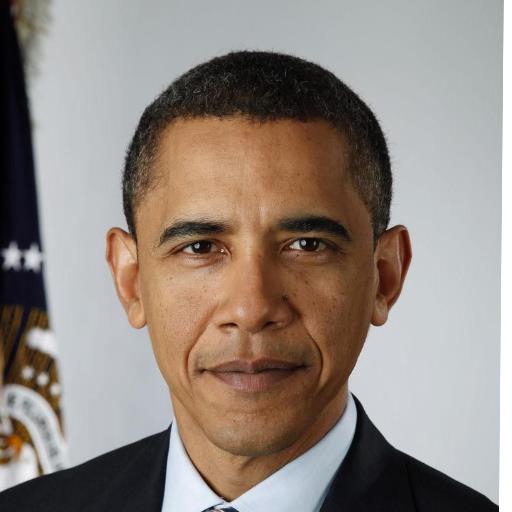
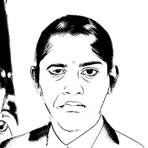
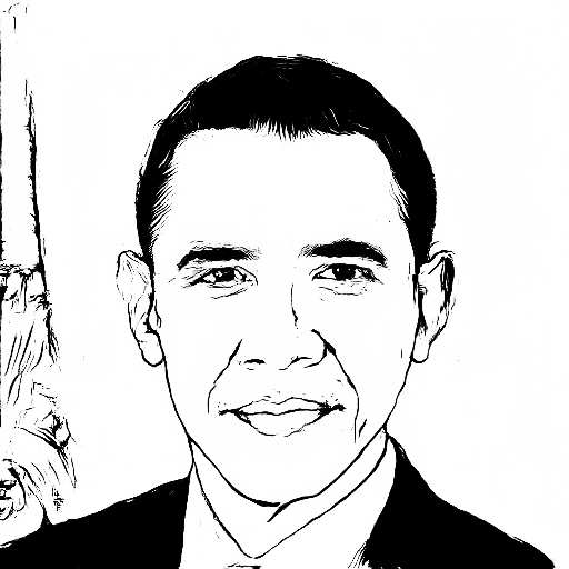
CoreThe premise is plain: a feasible solution actually obtained beats an optimum that cannot be obtained.

Chapter 8 · Coarse-to-fine

A model is only an approximation: a portrait, coarse to fine

A mathematical model of an engineering problem is only an approximation of the underlying complex system - just as even the most lifelike portrait is only an approximation of a photograph.

Obama Deep Image Analogy — (c) Deep Image Analogy

Portraits of Barack Obama by six methods: (a) input, (b) Gatys, (c) Deep Image Analogy, (d) CycleGAN, (e) Pix2Pix, (f) APDrawingGAN. Each ‘portrait’ is a different approximation of the same person - much like an engineering model is a different approximation of the real system (Yi et al., 2019).

Reference: Ran Yi, Yong-Jin Liu, Yu-Kun Lai, Paul L. Rosin. "APDrawingGAN: Generating Artistic Portrait Drawings from Face Photos with Hierarchical GANs." IEEE/CVF Conference on Computer Vision and Pattern Recognition (CVPR 2019), 10743–10752.

MeaningDo not read "finer model" as "truer model". Refinement removes one class of error; it never closes the gap between model and system.

Chapter 8 · Coarse-to-fine

Facility location: a textbook coarse model

Facility location is a classic problem of industrial engineering and logistics: place factories, warehouses or distribution centres to minimise cost or improve service.

Facility location: a coarse modelLet $J$ be candidate sites and $I$ customers; $x_j$ states whether facility $j$ is built and $y_{ij}$ whether customer $i$ is served by facility $j$.

\begin{aligned}\min\ & \sum_{j \in J} c_j x_j + \sum_{i \in I}\sum_{j \in J} h_{ij} y_{ij}\\\text{s.t.}\ & \sum_{j \in J} y_{ij} = 1,\quad \forall i \in I\\& y_{ij} \le x_j,\quad \forall i \in I,\; \forall j \in J\\& x_j,\, y_{ij} \in \{0,1\}\end{aligned}

Explicit cost: fixed construction cost $c_j$ and delivery cost $h_{ij}$ - both sit in the objective.
Implicit cost: workforce access and social-relation costs (a "not in my back yard" reaction to a waste plant or factory brings protests, bad press and permit delays, stretching the schedule and inflating public-relations spending) - none of them do.
Character: the model that internalises those further costs is the fine model; the coarse model is its simplified version.

Chapter 8 · Coarse-to-fine

Approximating the goal: from F(t-1) to F(t)

Suppose period $t-1$ is evaluated by the simplified goal $\mathcal{F}_{t-1}$ and period $t$ by $\mathcal{F}_t$, with $\mathcal{F}_t$ more complex. $\mathcal{P}_{t-1}$ is typically single-objective, linear and deterministic; $\mathcal{P}_t$ may become non-convex, nonlinear or uncertain.

Objective complexity rises in steps: every refinement pushes the problem into a harder class.

Chapter 8 · Coarse-to-fine

The approximation theorem: two inequalities that always hold

Let $X_t^\star$ be the optimum under $\mathcal{F}_t$ and $X_{t-1}^\star$ the optimum under $\mathcal{F}_{t-1}$. For a minimisation problem both of the following hold:

\[ \mathcal{F}_t(X_t^\star) \le \mathcal{F}_t(X_{t-1}^\star),\qquad \mathcal{F}_{t-1}(X_{t-1}^\star) \le \mathcal{F}_{t-1}(X_t^\star) \]

Insight 1When $\mathcal{F}_{t-1}(X_{t-1}^\star)=\mathcal{F}_{t-1}(X_t^\star)$, the stage-$(t-1)$ problem has multiple optimal solutions. Enumerate them, then evaluate with the richer $\mathcal{F}_t$ - far cheaper than solving $\mathcal{F}_t$ head-on.

Insight 2When $\mathcal{F}_t(X_t^\star) \lt \mathcal{F}_t(X_{t-1}^\star)$, $X_t^\star$ is a near-optimal solution under $\mathcal{F}_{t-1}$. Exploring near-optimal solutions at stage $t-1$ therefore pays off; Gurobi and CPLEX both expose multiple optima and solution pools.

Chapter 8 · Coarse-to-fine

The coarse phase and the fine phase

$\mathcal{M}_t$ is the model built at time $t$ with objective $\mathcal{F}_t$. Because $\mathcal{F}_t$ is closer to the real problem than $\mathcal{F}_{t-1}$, $\mathcal{M}_t$ is more complex than $\mathcal{M}_{t-1}$.

$\mathcal{M}_{t-1}$ is the coarse model and $\mathcal{M}_t$ the fine model; together the two phases form one round of coarse-to-fine.

Coarse phase: simplify the objective as far as possible (keep only some simple goals) and drop some complex constraints so the problem is tractable.
Fine phase: reuse the method built for $\mathcal{M}_{t-1}$ to construct a more faithful $\mathcal{M}_t$; feed its multiple and near-optimal solutions in as a warm start (or initial population).

Chapter 8 · Coarse-to-fine

The coarse-to-fine framework

The two phases compose into the framework below. The stopping rule belongs to the decision maker: a long development cycle may run ten rounds, a short one only one or two.

t = 0
while stopping conditions not met:          # coarse phase
    define a simplified objective  F(t-1)
    build the coarse model  M(t-1)
    develop a solution method for M(t-1)
    find all optimal solutions
    find near-optimal solutions
          # fine phase
    define a more complex objective  F(t)
    evaluate F(t) on the optimal and near-optimal solutions
    if a better solution is found:
        build the fine model  M(t)
        design a specialised method for M(t)
        t = t + 1
return the best solution

Note"Standing on the shoulders of giants" has a price in engineering: even a simple model costs serious time and money to solve, so the fine phase must reuse that investment rather than start over.

Chapter 8 · Coarse-to-fine

Case: the container relocation problem (CRP)

The CRP was published online by Kim and Hong in 2004 and in print in 2006; it has been studied for more than twenty years. When a target container sits beneath others, the containers on top must be temporarily relocated - at a cost in moves, time or equipment wear.

A bay of 3 stacks x 3 tiers. Target container 1 sits at the bottom of S1 under containers 2 and 6; because 6 lies above 2 it must move first, so at least 2 relocations are needed.

Blocked container: one that cannot be reached because others are stacked on top of it.
Relocation: temporarily moving a blocking container to another stack or an empty slot to free the target.

Chapter 8 · Coarse-to-fine

Three objectives for the CRP: a coarse-to-fine ladder

The original goal is to minimise yard-crane operating time $\mathcal{F}_c$. That quantity is hard to evaluate, so Kim and Hong approximated it by the total number of relocations $\mathcal{F}_a$; the crane travel distance $\mathcal{F}_b$ is also easier than $\mathcal{F}_c$.

All three objectives approximate the same goal, yet the resulting problem differs sharply in difficulty: $\mathcal{F}_a$ (2004, easy) to $\mathcal{F}_b$ (difficult) to $\mathcal{F}_c$ (2025, hard).

Key assumptionApproximating $\mathcal{F}_c$ by $\mathcal{F}_a$ implicitly assumes that fewer relocations imply a shorter crane distance. That assumption was never proved mathematically.

Chapter 8 · Coarse-to-fine

Multiple optima under F(a), and the distance criterion

Even though $\mathcal{F}_a$ is extremely simple, the CRP still has multiple optimal solutions under it: both plans below need 2 relocations, so $\mathcal{F}_a$ cannot tell them apart.

Using stack pitch 6.0 m, tier pitch 2.6 m and a 9.0 m clearance: option A covers 58.0 m and option B 34.0 m. Ranking the $\mathcal{F}_a$-optimal set by $\mathcal{F}_b$ picks the better plan.

MethodThis is exactly secondary optimisation of Chapter 9: $\min\{g(x): x \in \mathcal{S}^\star\}$ with $g=\mathcal{F}_b$. It is nearly free - just re-score solutions you already have.

Chapter 8 · Coarse-to-fine

Counterexample: the same operations, a different distance

Two yards start from different layouts, yet undergo exactly the same two relocations (move container 6 to S2, then container 2 to S3). The landing tier depends on how tall each stack already is, so the distances differ.

Layout 1 lands the boxes lower and totals 48.6 m; layout 2 lands them higher and totals 43.4 m. Same relocation count, different distance.

Conclusion"Fewer relocations imply a shorter distance" is therefore not always true. Approximating $\mathcal{F}_b$ by $\mathcal{F}_a$ is a lossy approximation - which is exactly why we proceed coarse-to-fine rather than in one leap.

Chapter 8 · Coarse-to-fine

Three insights

Using the container relocation problem as the thread, the chapter yields three conclusions that matter in practice.

A simple objective is not a simple answer. A complex problem with a simple objective is easy to solve, yet that objective may admit multiple optimal solutions - non-uniqueness is a resource, not a nuisance.
A more faithful objective is not a better solution. Moving to a richer $\mathcal{F}_t$ does not guarantee a better solution in reality - only a better one on the (still approximate) scale of $\mathcal{F}_t$.
Objectives must be weighed against the project timeline. Facing a new complex problem, the decision maker must balance the fidelity of the objective against the timescale of the project.

In one lineObtain a solution first, then complicate the objective - but never forget the objective is only a portrait of the system.

CHAPTER 9

Multiple solutions

Engineering often has more than one good solution; offering a basket beats betting on a single optimum.

Chapter 9 · Multiple solutions

Why a single optimum is not the end of the story

Most textbooks stop once the solver returns one optimal point $x^\star$. Engineering practice starts there: the model is a simplification of a far richer decision. Three facts make the *set* of good solutions more interesting than any single member.

The model is incomplete. Cost of implementation, operator workload, maintainability, safety margins, contractual flexibility - the model rarely prices any of them. Two solutions the model rates as equal can be very different on these omitted axes.
The model is symmetric. Identical machines, interchangeable facilities, permutable nodes make many distinct decisions score identically. The solver picks one arbitrarily.
The data are approximate. Every parameter is an estimate. A solution that wins by a hairline margin is fragile; a slightly worse one sitting in a wide basin of feasibility is safer.

PointAn optimizer returns one point; a decision maker needs an informed choice. The set of solutions that is essentially as good as the optimum is where the real engineering value lies.

Chapter 9 · Multiple solutions

Why engineering wants a basket, not a point

Mathematics shows the optimal and near-optimal sets can be large (9.3-9.7). The deeper reason engineers want that set - rather than the single point a solver returns - is decision-making, not algebra:

Left: a single optimum is isolated and narrow; the slightest deviation leaves optimum, even infeasibility. Right: the near-optimal set is wide and flat, so a disturbance keeps you near-optimal and feasible - exactly the resilience engineering wants.

Uncertainty & robustness. The nominal optimum $x^\star$ can violate constraints the moment reality departs from the model. A basket lets us keep the solution whose near-optimal neighbourhood stays feasible under every disturbance $\xi$.
Risk is not one number. We minimise expected regret $\mathbb{E}_\xi[f(x,\xi)-f^\star(\xi)]$ over a set, so a single bad realisation does not sink the whole plan.
The model omits the human. Maintainability, operator workload, safety culture and contractual flexibility are rarely priced. Among model-indistinguishable solutions the engineer picks the one those omitted axes favour.
Conflicting stakeholders. Cost, time and safety are weighed differently by different departments. A solution set supports negotiation instead of imposing one winner.
Contingency & option value. A pre-vetted alternative is ready when the field plan fails; preserving flexibility for tomorrow is itself worth money (value of flexibility).

Bottom line A single optimum is a mathematical artefact; a basket of good solutions is an engineering asset. We study $\mathcal{S}^\star$ and $\mathcal{S}_\varepsilon$ so the solver becomes a recommendation engine, not an oracle.

Chapter 9 · Multiple solutions

The optimal set and alternative optima

Before discussing multiple optima we need the set of *all* optima.

The optimal setFor the generic program $f^\star = \min_{x \in F} f(x)$ with feasible set $F \subseteq \mathbb{R}^n$:

\[ \mathcal{S}^\star = \bigl\{ x \in F : f(x) = f^\star \bigr\} \]

Alternative optimum: any $x' \in \mathcal{S}^\star$ with $x' \ne x^\star$. The cardinality of $\mathcal{S}^\star$ may be one (a unique optimum), finite (several isolated optima), or infinite (a continuum - for instance an entire edge or face of the feasible region).
Scope: linear and convex programs, combinatorial and mixed-integer models - any problem where the objective is indifferent between genuinely different decisions.
Character: which optimum a solver returns depends on implementation detail (branch order, degenerate pivots, pivoting rules), not on engineering meaning.

Chapter 9 · Multiple solutions

Where alternative optima come from: four sources

Almost every alternative optimum met in an engineering model comes from one of four sources.

Degeneracy in linear programming. Several distinct basic feasible solutions share one vertex and that vertex is optimal; simplex may also reach optimality through a series of degenerate pivots.
Redundant constraints. A constraint that is never active leaves slack the optimizer can trade off, producing families of optima.
Objective parallel to a face. When the objective gradient is orthogonal to a face, that entire face attains the same extreme value.
Structural symmetry. Interchanging identical resources - parallel lines, symmetric warehouse sites, permutable job families - yields optima that differ only by a relabelling.

Chapter 9 · Multiple solutions

The geometry of the optimal set: a convexity theorem

For the convex problems that dominate engineering optimization the structure of the optimal set is tightly constrained.

Theorem: optimal set of a convex programIf $F$ is convex and $f$ is convex, then the optimal set $\mathcal{S}^\star$ is convex (possibly a singleton, possibly empty). For a linear program

\[ \min\ \bigl\{ c^\top x : Ax \ge b,\; x \ge 0 \bigr\} \]

$\mathcal{S}^\star$ is a face of the feasible polytope; whenever its dimension exceeds zero it contains uncountably many optimal solutions.
Scope: convex and linear programs, and the large class of engineering models that can be convexified.
Character: this is why an LP solver may legitimately return *any* optimum: the set is convex, so averaging two optima yields a third.

Corollary: two optima are enough to manufacture infinitely more - the basis of the post-optimality procedures below.

Chapter 9 · Multiple solutions

Secondary optimisation: choosing among optima

"The model says these are equally good" is not the end but the start of the question: if the model cannot discriminate, use a criterion from outside it.

Secondary optimisationWhen many $x$ attain $f^\star$, the engineer is free to choose among them with a secondary criterion $g(x)$:

\[ \min_{x}\ g(x)\quad \text{s.t.}\quad x \in \mathcal{S}^\star \]

Equivalently, the lexicographic problem that minimises $f$ first and, only among optimal $f$, minimises $g$.
Typical uses: among optimal production plans take the one with least total setup/changeover time; among optimal network designs open the fewest facilities (easier to run and audit); among optimal schedules maximise slack on the critical path (most resilient to breakdown).

EnumerationIteratively cut off the incumbent and re-solve. For binary variables use the Hamming cut $\sum_{j: x_j^\star=1} x_j + \sum_{j: x_j^\star=0}(1-x_j) \le n-1$; for continuous problems perturb the objective plane slightly.

Chapter 9 · Multiple solutions

Illustration: an edge of optima

Take $P=\{x \ge 1,\; x \le 5,\; y \ge 1,\; x+3y \le 17,\; 2x-y \ge -1\}$ and minimise $f=y$. The objective contours are parallel to the lower edge, so every point of that edge is optimal - not just its two endpoints.

The model is indifferent between $x^{(1)}$, $x^{(2)}$ and everything in between; the engineer is not. Maximising the *minimum slack* as a secondary criterion puts the best choice at $x=(3.00, 1)$ with slack 2.00, against only 0.00 at the endpoints $(1,1)$ and $(5,1)$.

Reminder$f^\star = 1$ and there are infinitely many optima. Which endpoint the solver returns is an implementation detail, not an engineering conclusion.

Chapter 9 · Multiple solutions

The near-optimal set and epsilon-optimality

In practice the model error is itself of order $\varepsilon$. Insisting on the singleton optimum while ignoring a whole $\varepsilon$-neighbourhood is statistically indefensible.

$\varepsilon$--optimalityThe gap between the optimum and a slightly worse solution is rarely meaningful next to the model error, so we enlarge the target set:

\[ \mathcal{S}_{\varepsilon} = \bigl\{ x \in F : f(x) \le f^\star + \varepsilon \bigr\},\qquad \varepsilon \ge 0 \]

For $\varepsilon=0$ this recovers $\mathcal{S}^\star$. The size of $\varepsilon$ should track the fidelity of the model: if the data are known only to within a few percent, demanding more from the optimum is false precision.
Character: if $F$ and $f$ are convex, $\mathcal{S}_{\varepsilon}$ is convex for every $\varepsilon \ge 0$ (an intersection of two convex sets).

Chapter 9 · Multiple solutions

Why near-optimal solutions carry the real value

Three properties make the near-optimal set the practical prize.

Structural diversity. Near-optimal solutions are often not small perturbations of one another; they can activate different constraints, open different facilities, pick different topologies. That variety is what lets a secondary goal be met almost for free.
Robustness and flexibility. A solution surrounded by a wide feasible $\varepsilon$-neighbourhood is more stable than one perched on a sharp peak; small data perturbations are less likely to wreck it.
A bridge to multi-objective thinking. Relaxing the single objective by $\varepsilon$ and exploring the resulting set is exactly how one begins to trade the primary goal against the others.

Chapter 9 · Multiple solutions

Generating a diverse solution pool

Modern solvers maintain a solution pool: a ranked collection of distinct feasible solutions. CPLEX populate, Gurobi PoolSearchMode / PoolSolutions and SCIP all enumerate diverse solutions within a gap of the optimum.

solve P  ->  f*
add the epsilon-constraint  f(x) >= f* - epsilon
pool = {x*}
while |pool| < K and feasible solutions remain:
    add a diversity cut excluding anything within r of a member of pool
    re-solve the extended problem
    if a new feasible x' is found:  pool = pool + {x'}
    else: break
return pool

Exhaustive enumeration of a 0-1 knapsack with capacity 58: optimum $f^\star=122$ with 16 optima; allowing $\varepsilon=4$ (at most 3.3% loss) gives a pool of 54 solutions whose "number of distinct suppliers" ranges from 2 to 4 - the primary objective barely moves while the secondary cost differs by 2 suppliers.

Chapter 9 · Multiple solutions

Connections to the rest of the book

"Multiple solutions" is not a standalone trick; it is a thread running through the whole book.

Coarse-to-fine (Chapter 8): a pool of near-optimal candidates from the relaxed model feeds the refinement stage - precisely the $\mathcal{S}_{\varepsilon}$ of this chapter.
Robust optimisation (Chapter 11): prefer the solution whose near-optimal neighbourhood stays feasible under every realisation of the uncertainty.
Multi-objective optimisation (Chapter 13): generalises the idea - not one $\varepsilon$-band but the full trade-off (Pareto) surface.
Matheuristics and metaheuristics (Chapters 18-20): maintaining and improving a near-optimal pool is their central data structure.

Chapter 9 · Multiple solutions

Case: a solution pool for one knapsack

Capacity 58 with 10 items, enumerating all $2^{10}=1024$ subsets: optimum $f^\star=122$ with 16 optima; relaxing by $\varepsilon=4$ gives a pool of 54 solutions.

Optimum: $f^\star = 122$ with 16 optima - the solver hands you exactly one of them.
Near-optimal pool: 54 solutions at $\varepsilon=4$, losing at most 4 (3.3%) on the primary objective.
What the secondary criterion buys: with $g$ = number of product lines the pool spans 2 to 4; taking the $g=2$ solution removes 2 suppliers for at most 4 on the primary objective.

ReadingThe model error is already of order $\varepsilon$. Optimising a secondary goal inside the $\varepsilon$-band means trading precision the model cannot see for value the model did not count.

Chapter 9 · Multiple solutions

Case: enumerating alternative optima with the Hamming cut

Repeatedly cut-and-resolve on the same knapsack pulls out distinct optima one by one: (p=122, w=58, items 2,3,6,8,9,10) → (p=122, w=58, items 1,2,4,5,6,9) → (p=122, w=58, items 1,2,4,5,7,9).

\[ \sum_{j: x_j^\star = 1} x_j + \sum_{j: x_j^\star = 0} (1 - x_j) \le n - 1 \]

The cut removes only the incumbent $x^\star$ and leaves $\mathcal{S}^\star \setminus \{x^\star\}$ intact.
If the re-solve returns the same objective value, an alternative optimum has been found; repeat.
For continuous problems perturb the objective plane instead; Gurobi and CPLEX ship this workflow as a ready-made API.

Chapter 9 · Multiple solutions

Exercise: a secondary choice along the optimal edge

Back to the polygon of the earlier slide. $f^\star=1$ and the optimal set is the whole segment $\{(x,1): 1 \le x \le 5\}$. Now take "maximise the minimum slack" as the secondary criterion $g$.

The four slacks are $17-x-3y$, $2x-y+1$, $5-x$ and $x-1$; on the optimal edge $y=1$, take their minimum.
Both endpoints $(1,1)$ and $(5,1)$ have minimum slack 0.00 - they hug the constraint boundary and can turn infeasible if the data shift.
The point $(3.00, 1)$ reaches minimum slack 2.00, the most perturbation-tolerant point on the edge.

ConclusionSame $f^\star$, different engineering consequences. Whether the solver reports $(1,1)$ or $(5,1)$ is chance, but the most tolerant point is $(3.00, 1)$ - a conclusion only the secondary criterion can deliver.

Chapter 9 · Multiple solutions

Chapter summary

A single optimal point is the beginning, not the end, of engineering decision-making.

The optimal set $\mathcal{S}^\star$ and, more usefully, the near-optimal set $\mathcal{S}_{\varepsilon}$ contain many solutions the model cannot distinguish but the engineer can.
For convex and linear programs both sets are convex (a face of the polytope in the LP case), which makes them easy to characterise and to sample.
Enumerating alternative optima with exclusion cuts, or populating a diverse pool, turns an opaque solver into a transparent recommendation engine.
Among essentially equivalent solutions, pick the one that is cheapest to implement, most robust, or fairest.

In one lineWhen the model says "any of these is optimal", the engineer should ask: "which one is best for the world the model forgot?"

Part III

Engineering Optimization Problems

What a problem looks like often decides which method you can use. This part classifies by structure: deterministic/combinatorial, robust, bilevel, multi-objective, multi-stage, game.

第三部分 · 工程优化问题

本篇逻辑框架

问题长什么样，往往决定了你能用什么方法。本篇按结构把问题分类：从确定性 / 组合，到鲁棒、双层、多目标、多阶段与竞争博弈。

逻辑主线：沿“确定 → 不确定”“单主体 → 多主体”“单阶段 → 多阶段”三轴展开，七章覆盖主要问题结构谱系。

CHAPTER 10

Deterministic / Combinatorial

Whether variables are continuous or discrete, and structure decomposable or tightly coupled, decides if the problem lands in P or NP-hard.

Chapter 10 · Deterministic / Combinatorial

Continuous: LP and NLP

Continuous optimization uses real variables. Linear programming (LP) has linear objective and constraints, solved in polynomial time by simplex/interior-point; nonlinear programming (NLP) allows nonlinear terms and is far harder.

LP canonical: min c^T x s.t. A x <= b, x >= 0. Convex NLP may still be globally solvable; nonconvex gives only local guarantees.

Concrete form (transportation LP)

\[ \min\ \sum_{i,j} c_{ij}x_{ij}\quad\text{s.t.}\quad \sum_j x_{ij}=a_i\ (\forall i),\ \sum_i x_{ij}=b_j\ (\forall j),\ x_{ij}\ge 0 \]

E.g. 2 sources (capacity 20,30), 2 sinks (demand 25,25), cost matrix $\begin{pmatrix}3&5\\4&2\end{pmatrix}$. This is the abstract $\min c^\top x,\ Ax\le b$ of s-c10a made concrete: continuous variables, linear constraints, hence polynomial.

Chapter 10 · Application

Application: feed blending is an LP

A typical continuous-optimization application: minimise cost under proportionality and additivity constraints. The LP below is exactly the continuous problem of s-c10a, made concrete.

Concrete model (feed blending)

\[ \min\ 3x_1+5x_2 \quad\text{s.t.}\quad 2x_1+x_2\ge 8,\; x_1+3x_2\ge 9,\; x_1,x_2\ge 0 \]

Two ingredients $x_1,x_2$ (tonnes) at cost 3/5; constraints are lower bounds 8 on protein and 9 on fibre. The optimum sits at a polyhedron vertex: simplex reaches it in one pivot, with $x_1=3,\;x_2=2$, cost 19. Relax either bound and the feasible region shifts and the vertex moves - the intuition behind "continuous, linear, polynomial".

Takeaway Once a continuous problem is an LP, polynomial guarantees exist; the hard part is modelling (does proportionality hold?), not solving.

Chapter 10 · Deterministic / Combinatorial

Integer and combinatorial

When variables must be integers or discrete choices (location, scheduling, routing), problems usually become NP-hard. This is the most common hard case in engineering optimization.

0-1 variables encode yes/no decisions (build this warehouse or not).
Combinatorial blow-up: n binary variables give 2^n combinations.
Exact methods (branch-and-bound) prove optimality but scale poorly; heuristics trade for speed.

Concrete form (0-1 knapsack)

\[ \max\ \sum_j p_j y_j\quad\text{s.t.}\quad \sum_j w_j y_j\le W,\ y_j\in\{0,1\} \]

E.g. capacity $W=8$, items $(p,w)=(6,2),(10,4),(12,5)$. Enumerate $2^3=8$; optimum $y=(1,0,1)$, value 18, weight 7. This is the "$2^n$ combinations from n binary variables" of s-c10b made concrete.

Chapter 10 · Combinatorial

Case: one-dimensional cutting stock

6,000 mm stock bars, 33 pieces in four lengths. Filling each bar as full as possible (first-fit decreasing) is the natural greedy, but it cannot see patterns.

Lower bound: 47,050 / 6,000 → at least 8 bars.
The FFD greedy uses 9 bars, 12% above optimal.
Optimum is 8 bars (950 mm trim, only 2.0%): 3 bars of (2200+2×1300+950), 3 of (1850+1300+3×950), 2 of (2200+2×1850).

The decision variable is the cutting pattern, not "which piece goes on which bar". Once you count patterns instead of pieces, column generation applies.

Chapter 10 · Deterministic / Combinatorial

Network flow problems

Many engineering problems are flows on graphs: shortest path, max flow, min-cost flow. Their special structure admits efficient, often polynomial algorithms.

Lesson: recognize a problem as network flow first, and you may dodge the expensive general MIP solve.

Concrete form (min-cost flow)

\[ \min\ 2x_{SA}+5x_{ST}+1x_{AT}\quad\text{s.t.}\quad x_{SA}+x_{ST}=12,\ x_{SA}=x_{AT},\ 0\le x\le 10 \]

E.g. source S supplies 12, sink T needs 12; arcs S→A (cap 10, cost 2), S→T (cap 5, cost 5), A→T (cap 10, cost 1). Optimum saturates S→A→T with 10 and S→T with 2, cost 30. This is the abstract conservation form of s-c10c made concrete.

Chapter 10 · Combinatorial

Case: cold-chain warehouse network (fixed-charge design)

Three candidate DCs, four demand cities. Opening a DC costs a fixed charge; freight varies by lane. Two common intuitions are both wrong here.

Intuition 1 "open the cheapest DC": Xi’an alone costs 11,000 — the worst option on the board.
Intuition 2 "more is safer": all three open costs 8,880, which is 240 above optimal.
The optimum is Wuhan + Xi’an at 8,640. The fixed charge makes the objective non-monotone, so every subset must be compared.

Fixed charge plus linear freight is a mixed-integer program. Its feasible set is a union of discrete pieces, so every gradient-flavoured intuition fails.

Chapter 10 · Deterministic / Combinatorial

Scheduling problems

Scheduling sequences who does what when, the home of combinatorial optimization: job-shop, vehicle routing, and terminal operations all live here.

Single/parallel machine: relatively tractable.
Flow/job shop: strongly NP-hard.
With time windows and resource constraints: realistic but harder.

Concrete form (2-machine flow shop)

\[ \min\ C_{\max}\quad\text{s.t.}\quad C_{\max}\ge p_{1,\pi(k)}+p_{2,\pi(k)}+\sum_{\ell

E.g. 3 jobs, times $P=\begin{pmatrix}3&2\\4&1\\2&3\end{pmatrix}$ (rows=jobs, cols=machines 1/2). Johnson's rule gives order (1,3,2), makespan 11; a careless order reaches 13. This is the abstract scheduling form of s-c10d made concrete.

Chapter 10 · Combinatorial

Case: job-shop scheduling (disjunctive graph)

Each job is a sequence of operations, processed in machine order.
Conjunctive arcs fix operation order; disjunctive arcs choose one ordering per machine.
Choosing all disjunctive arcs yields an acyclic schedule — exactly the combinatorial difficulty.

The disjunctive graph paints scheduling as machine conflicts waiting to be ordered; each resolved arc brings a feasible schedule closer.

Chapter 10 · Deterministic / Combinatorial

How structure decides tractability

The same minimization goal can be trivial or intractable purely by structure. Identifying structure is job one.

Good structure: convex, network, tree, submodular, often efficient or approximable.

Bad structure: nonconvex, tightly coupled, hard symmetry breaking, often needs heuristics or exact backstop.

Chapter 10 · Deterministic / Combinatorial

Three orthogonal classification axes

Deterministic problems are classified along axes that decide which tool to reach for.

By model shape (linear vs nonlinear)

Linear → LP: simplex / interior-point, polynomial time.
Nonlinear → NLP; convexity decides local = global.

By constraints (constrained vs unconstrained)

Unconstrained → calculus / gradient search.
Constrained → capacity, safety, regulation make it real.

By variable type (continuous vs combinatorial)

Real-valued → smooth feasible region.
Integer / binary → combinatorial explosion.

Chapter 10 · Deterministic / Combinatorial

The MIP: unifying model of combinatorial problems

\[ \min_{x,y}\; c^{\top} x + d^{\top} y \quad\text{s.t.}\quad A x + B y \ge b,\; x_j\in\mathbb{Z}_{+},\; y_k\in\{0,1\} \]

Here $y$ encodes discrete choices (assign, sequence, select) and $x$ the continuous quantities coupled to them. This single form underlies berth allocation, crane scheduling, routing and storage.

Chapter 10 · Deterministic / Combinatorial

Five combinatorial archetypes

Archetype	Decision	Terminal instance
Assignment	one-to-one matching under cost	Quay crane ↔ berth section
Scheduling	order tasks on resources over time	Quay-crane load/unload sequence
Routing	visit nodes at minimum travel cost	AGV / yard-truck paths
Packing / cutting	fit items into capacitated bins	Container stowage, yard-block filling
Network design	choose cheapest arcs / nodes	Terminal layout, transshipment links

Each archetype hides an explosion: $n$ jobs → $n!$ permutations; $n$ nodes → $(n-1)!/2$ tours.

Chapter 10 · Combinatorial

Case: a terminal as five combinatorial archetypes

LP/NLP (continuous), IP/MIP (integer), network flow, scheduling, routing.
One terminal contains all five — and they couple to each other.
Structure decides tractability: the hardest class is usually the bottleneck.

Decomposing the terminal into five archetypes makes it clear: continuous parts are easy; integer and routing parts are the NP-hard root.

Chapter 10 · Deterministic / Combinatorial

Why hard: integrality gap & NP-hardness

Integrality gap. The LP relaxation bounds the integer optimum; for the assignment problem the matrix is totally unimodular, so the relaxation is already integer-optimal.
NP-hardness. TSP, bin-packing and most sequencing problems are NP-hard: no polynomial algorithm unless P = NP.
Engineering reading. NP-hardness forbids a guarantee of optimality in polynomial time — blend exact (small) with heuristic (large).

Chapter 10 · Deterministic / Combinatorial

Canonical forms: continuous and integer problems

The dividing line in this chapter is whether a variable may take fractional values. That single choice decides polynomial solvability or NP-hardness.

Linear program (LP)定义：Objective and every constraint are linear in the decision variables, which are continuous.

\[\min_{x}\; c^{\top}x \quad\text{s.t.}\quad Ax \ge b,\; x \ge 0\]

适用范畴：Blending, transport, capacity allocation — whenever proportionality and additivity hold.
特点：The feasible set is a polyhedron and an optimum sits at a vertex; solvable in polynomial time, strong duality holds, and duals are shadow prices.

Nonlinear program (NLP)定义：The objective or a constraint is nonlinear, while the variables stay continuous.

\[\min_{x}\; f(x) \quad\text{s.t.}\quad g_j(x)\le 0,\; h_i(x)=0,\; x\in\mathbb{R}^{n}\]

适用范畴：Physical laws (drag, energy), geometric design, risk and utility — anything with products or power laws.
特点：For a convex NLP (f and g convex, h affine) a KKT point is globally optimal; otherwise only local optimality is guaranteed.

Mixed-integer program (MIP)定义：Some or all variables are restricted to integers (often 0-1) to express discrete choices, logic and fixed charges.

\[\min_{x,y}\; c^{\top}x + d^{\top}y \quad\text{s.t.}\quad Ax+By \ge b,\; x\in\mathbb{Z}_{+}^{n},\; y\ge 0\]

适用范畴：On/off, select-or-not, batching, rostering, routing — any yes/no decision.
特点：NP-hard; the LP relaxation gives a bound that branch-and-bound and cuts tighten. The integrality gap measures the relaxation, and modelling choices (symmetry, big-M tightness) drive solve time.

Made concrete (LP / NLP / MIP)

\[\begin{aligned}\text{LP:}&\ \min\ 4x_1+3x_2\ \text{s.t.}\ x_1+2x_2\ge 8,\ 3x_1+x_2\ge 9,\ x\ge0;\\\text{NLP:}&\ \min\ x^2+y^2\ \text{s.t.}\ x+y=1\ \Rightarrow\ (0.5,0.5);\\\text{MIP:}&\ \min\ 5y_1+8y_2\ \text{s.t.}\ 3y_1+5y_2\ge 7,\ y\in\{0,1\}^2\ \Rightarrow\ y=(1,1).\end{aligned}\]

The abstract $c^\top x$, $f(x)$, $(c^\top x+d^\top y)$ become specific coefficients; the LP vertex, the NLP KKT point and the MIP 0-1 choice are all explicit.

Chapter 10 · Deterministic / Combinatorial

Networks, scheduling and structure

Both are combinatorial, yet structure decides fate: network flow is easy thanks to total unimodularity, scheduling is hard because of permutations.

Network flow problem定义：Choose arc flows on a directed graph that satisfy flow conservation and capacity limits at minimum cost.

\[\min\ \sum_{(i,j)\in A} c_{ij}x_{ij}\quad\text{s.t.}\quad \sum_{j}x_{ij}-\sum_{j}x_{ji}=b_i\ \forall i,\quad 0\le x_{ij}\le u_{ij}\]

适用范畴：Transport, transshipment, assignment, shortest paths, max-flow/min-cut, multi-echelon supply chains.
特点：The constraint matrix is totally unimodular, so the LP relaxation is automatically integral — an integer problem that is polynomial, with strongly polynomial algorithms available.

Scheduling problem定义：Assign jobs to resources and order them over time to optimise completion time, tardiness or throughput; classified by the Graham triplet $\alpha|\beta|\gamma$.

\[\min_{\pi}\ \sum_{j=1}^{n} w_j C_j,\qquad C_{\pi(k)}=\sum_{\ell=1}^{k} p_{\pi(\ell)}\]

适用范畴：Shop floors, quay cranes, operating theatres, compute clusters, project planning.
特点：NP-hard apart from a few structures where simple rules (SPT, WSPT, EDD) are optimal. Modelled with disjunctive graphs and solved by priority rules or metaheuristics; adding setups, due dates or availability changes tractability.

Made concrete (network / scheduling)

\[\begin{aligned}\text{flow:}&\ \min\ 2x_{SA}+x_{AT}\ \text{s.t.}\ x_{SA}=x_{AT}=12,\ 0\le x\le 10\ (\text{cost }30);\\\text{sched:}&\ 3\text{ jobs }P=\begin{pmatrix}3&2\\4&1\\2&3\end{pmatrix},\ \text{Johnson order }(1,3,2),\ C_{\max}=11.\end{aligned}\]

The abstract conservation form and the Graham triplet become concrete arc flows and a concrete processing-time matrix; "totally unimodular → polynomial" and "permutations → NP-hard" get a computable contrast.

Chapter 10 · Combinatorial

A small example: the 4-node travelling salesman problem

Combinatorial problems: variables are restricted to a finite set (which machine, route, or bay).
A 4-city TSP has only (4−1)!/2 = 3 distinct tours — small enough to enumerate.
Slightly larger and it explodes: n binary decisions yield up to 2ⁿ configurations.
This is the workhorse of logistics and manufacturing: B&B proves optimality, metaheuristics scale.

The difficulty of combinatorial problems is not modelling but the exponentially growing search space.

Chapter 10 · Combinatorial

Case: airport gate assignment (the greedy trap)

Six flights, three gates, minimise passenger walking. Giving the nearest free gate to the earliest flight is the worst thing you can do: a long-stay flight locks up the near gate all day.

Flight F1 stays 5.5 h. Parking it at the near gate pushes the five short flights out to the far gates.
The optimum is the reverse: the long stay goes to B (260 m), all five short stays keep A (120 m).
A gap of 39,200 passenger-metres: greedy is 32.2% worse than optimal.

Same assignment problem, a different "reasonable" rule, 32% more cost. In combinatorial problems, local rules have almost no safety margin.

CHAPTER 11

Robust Optimization

Data are never exact. Robust optimization targets the worst case still acceptable, trading conservatism for reliability.

Chapter 11 · Robust Optimization

Model first, then uncertainty: from MIP to an uncertainty model

Optimization problems usually start as a mixed-integer program (MIP). Once some coefficients are uncertain, the same model becomes one that decides over an uncertainty set.

Abstract MIP model

$\min_{x,y}\; c^\top x+d^\top y$

$\text{s.t. } A x+B y\;\ge\; b$

$x\ge0,\;x\in\mathbb{R}^n;\; y\in\{0,1\}^p$

Continuous $x$ and 0–1 $y$ jointly decide feasibility and cost.

Corresponding uncertainty model

$(A,b)\;\leadsto\;(\tilde A,\tilde b)$

$(\tilde A,\tilde b)\in\mathcal{U}$

$x,y\text{ 须 }\forall(\tilde A,\tilde b)\in\mathcal{U}\text{ 可行}$

Not one $(A,b)$ but a whole family; the decision must survive the whole family.

Ex.1 · Capacity: output $x$, demand $\tilde d$ uncertain. If $\tilde d\in[80,120]$, require $x\ge\tilde d$ for every possible demand.

Ex.2 · Portfolio: allocation $y$, return $\tilde r$ uncertain. If only the range of $\tilde r$ is known, guarantee the worst case still meets target.

How much we know about the uncertainty decides the method — the division of labor for the rest of the book:

Only a point estimate (e.g. demand=100) → deterministic optimization: simple but fragile.
A known distribution (e.g. demand 80/100/120 each 1/3) → Stochastic Programming: optimize expectation, see Ch.15.
Only a range / set, no distribution (e.g. demand∈[80,120]) → Robust Optimization: guard the worst case, this chapter.

Chapter 11 · Robust Optimization

The robust counterpart

Ordinary optimization fixates on the nominal value (say demand = 100) and optimizes there; yet when the true demand is 120 the plan can collapse. Worse, a constraint must hold "for every value in $\mathcal{U}$" — infinitely many constraints, impossible to list.

The robust counterpart is the tractable re-writing: it turns "feasible for every case" into an optimization with a $\max$ — an opponent picks the worst case, your master problem defends against it.

Form: min_x max_{u in U} f(x,u) s.t. g(x,u) <= 0 for all u in U.

Example: a constraint $a x\le b$ with $a\in[8,12]$. Demanding it for a=8,9,10,11,12 is, by linearity, equivalent to guarding only the worst a=12, i.e. $12x\le b$.

Chapter 11 · Robust Optimization

Budget uncertainty sets

The shape of U sets the conservatism. A budget set caps the total simultaneous deviation, the most common compromise.

Why not the box? The box assumes every parameter hits its worst at once, so the plan is needlessly over-protected. The budget set (Bertsimas–Sim) allows at most $\Gamma$ parameters to deviate.

Budget set: sum |u_i - u_bar_i| / Delta_i <= Gamma. Larger Gamma is more conservative; Gamma=0 recovers deterministic optimization.

Example: three demands, nominal $\bar d_i=100$, swing ±20. Stock $x$ with $x\ge d_1+d_2+d_3$ for all cases. Box set → worst 120+120+120, need $x\ge 360$; budget set $\Gamma=1$ → at most one deviates, only $x\ge 320$.

Think of $\Gamma$ as an error-tolerance dial: 0 bets everything nominal, n pays for everyone-worst.

Chapter 11 · Robust Optimization

The conservatism trade-off

Robustness is not free: the more conservative, the worse the average performance and the more resources wasted. Gamma is the knob engineers must set.

Low Gamma: hugs nominal, cheap but volatility-fragile.
High Gamma: shock-resistant but chronically over-provisioned.

Chapter 11 · Robust Optimization

A robustness example

Take stowage: draft and stability constraints depend on cargo-density estimates with error. A budget set wrapping the error yields a plan that still satisfies stability under real density variation.

Cost: versus the nominal plan, about 3 percent more capacity buys the guarantee of safety under any plus-minus 5 percent density error.

Chapter 11 · Robust Optimization

Two philosophies under uncertainty

Under uncertainty two mainstream routes place different bets: stochastic programming bets on a known distribution, robust optimisation on a known range.

Stochastic programming

Assumes the distribution of the random vector ξ is known (or estimable from data).
Optimises the expected total cost.
Weakness: a misspecified distribution biases the solution systematically.
Use when: rich history, trustworthy distribution, repeated decisions (inventory, generation, unit commitment).
Example: emergency inventory. Order x first; demand ξ has a distribution; SP minimises expected cost.

Robust optimization

Only requires parameters to lie in an uncertainty set $\mathcal{U}$; no distribution needed.
Optimises the worst case over $\mathcal{U}$.
Guarantees feasibility for every $u\in\mathcal{U}$, distribution-free.
Use when: scarce data and hard-to-violate limits (safety, service guarantees, disaster response).
Example: demand d in [80,120]; requiring x≥d for all d in U forces x=120 — costliest in the worst case, yet never short.

Chapter 11 · Robust Optimization

Robust counterpart & uncertainty sets

\[ \min_{x\in X}\;\max_{u\in\mathcal{U}}\; f(x,u) \]

A larger $\mathcal{U}$ gives stronger protection but a more conservative (costlier) solution. Three standard shapes:

Box

$|u_j-\bar u_j|\le \hat u_j$

Independent intervals; often too pessimistic, over-protective.

Ellipsoidal

$(u-\bar u)^{\top}\Sigma^{-1}(u-\bar u)\le\rho^2$

Couples parameters via covariance; avoids worst extremes.

Budget (Bertsimas–Sim)

$\sum_j z_j\le \Gamma$

$\Gamma$ interpolates between nominal ($\Gamma=0$) and the full box; the usual compromise.

Chapter 11 · Robust Optimization

Bertsimas–Sim linearization

A budgeted-uncertain linear constraint becomes a small set of linear constraints — so the whole robust LP stays an LP.

\[ \sum_j \bar a_j x_j + \Gamma s + \sum_j p_j \le b,\qquad s + p_j \ge \hat a_j x_j,\quad p_j\ge 0 \]

Protecting one constraint costs only one extra variable $s$ and $n$ variables $p_j$.

Chapter 11 · Robust Optimization

Adjustable RO & choosing the budget Γ

\[ \min_{x\in X}\;\max_{u\in\mathcal{U}}\;\min_{y\in Y(x,u)} f(x,y,u) \]

Adjustable RO (ARO). Some decisions ($y$) are made after observing $u$; an affine decision rule $y(u)=y^0+\sum_k y^k u_k$ keeps it tractable.
Engineering point. The budget $\Gamma$ is calibrated on historical data — choosing it often matters more than the solver.

Chapter 11 · Uncertainty

Three paradigms for uncertainty

They differ in what you know about the distribution: you know it, you only know a range, or you only have samples.

Stochastic program (SP)定义：Assumes the distribution of the random vector $\xi$ is known (or estimated) and optimises expected cost.

\[\min_{x}\; c^{\top}x + \mathbb{E}_{\xi}\big[\,Q(x,\xi)\,\big],\qquad Q(x,\xi)=\min_{y}\{\,q^{\top}y:\; Wy \ge h(\xi)-T(\xi)x\,\}\]

适用范畴：Rich history, trustworthy distributions, repeated decisions: inventory, capacity, generation and unit commitment.
特点：Interpretable (expected cost), but scenarios explode with the horizon, so sampling or decomposition (L-shaped) is needed; a misspecified distribution biases the solution systematically.

Robust optimisation (RO)定义：No distribution is assumed: the solution must be feasible for every realisation in an uncertainty set $U$, and the worst case is optimised.

\[\min_{x}\ \max_{\xi\in U}\ f(x,\xi)\qquad\text{s.t.}\qquad g(x,\xi)\le 0\ \ \forall\,\xi\in U\]

适用范畴：Scarce data and hard-to-violate limits: safety constraints, service guarantees, disaster response.
特点：Often tractable (box sets dualise to linear; budget sets linearise) at the price of conservatism. Choosing the uncertainty set is modelling the risk appetite.

Distributionally robust optimisation (DRO)定义：In between: the true distribution is unknown but confined to an ambiguity set $\mathcal{D}$ (moment constraints, or a Wasserstein ball around the empirical distribution), and the worst-case expectation is optimised.

\[\min_{x}\ \sup_{P\in\mathcal{D}}\ \mathbb{E}_{P}\big[\,f(x,\xi)\,\big]\]

适用范畴：Samples exist but you refuse to bet on one distribution: small-sample inventory, machine learning, finance.
特点：Less conservative than RO (it uses distributional information) and more robust than SP (no single distribution is trusted); moment or Wasserstein ambiguity sets keep it tractable.

Chapter 11 · Uncertainty

Chance constraints and the shape of uncertainty sets

The shape of the uncertainty set determines what the robust counterpart becomes after dualisation, and hence how hard the problem is.

Chance-constrained program (CCP)定义：Small violations are allowed: a constraint holds with probability at least $1-\alpha$.

\[\min\ c^{\top}x\qquad\text{s.t.}\qquad \mathbb{P}\big(\,g(x,\xi)\le 0\,\big)\ \ge\ 1-\alpha\]

适用范畴：Service levels, reliability, stock-out rates, N-1 security — anywhere occasional violation is tolerable.
特点：Intuitive semantics, but the feasible set is usually non-convex; exact treatment needs special distributions or scenarios with big-M, otherwise one uses sampling (SAA) or conservative convex approximations such as CVaR.

Three canonical uncertainty sets定义：Box (everything at its worst), ellipsoidal (captures correlation), budget (bounds how many parameters deviate at once).

\[U_{\infty}=\{\xi: \lVert\xi-\hat\xi\rVert_{\infty}\le \rho\},\quad U_{2}=\{\xi: \lVert\Sigma^{-1/2}(\xi-\hat\xi)\rVert_{2}\le \Omega\},\quad U_{\Gamma}=\{\xi: \sum_j \frac{|\xi_j-\hat\xi_j|}{\hat\xi_j}\le \Gamma\}\]

适用范畴：Box for worst-case analysis, ellipsoidal when covariance is known, budget when "everything worst at once" is simply unrealistic.
特点：Sweeping $\Gamma$ from 0 to n traces a conservatism curve from the nominal to the box solution; the ellipsoidal set dualises to a second-order cone. All three stay computationally tractable.

Chapter 11 · Robust

Case: the budget uncertainty set (Γ)

Box set: every parameter varies within ±% independently — too conservative.
Budget set: at most Γ parameters deviate at once; the rest stay nominal.
Larger Γ is more conservative, smaller is closer to deterministic — conservatism is tunable.

The box allows all parameters worst at once; the budget set allows only Γ of them, sharply tightening conservatism.

Chapter 11 · Robust

Case: berth allocation under uncertainty

Arrival times vary — the nominal plan is packed tight and a single delay cascades.
The robust plan inserts buffers between vessels, trading some efficiency for stability.
This is the determinism vs speed trade-off seen through a robustness lens.

The nominal plan packs vessels for throughput; the robust plan inserts buffers to absorb delay — the efficiency/stability swap.

Chapter 11 · Robust

Uncertainty sets: box / ellipsoid / budget Γ

Robust optimization protects against the worst case over an uncertainty set, not a distribution.
Box: each parameter bounded independently — simple but often too conservative.
Ellipsoid: captures Gaussian-like perturbations, moderate conservatism.
Budget set Γ (L1): at most Γ parameters deviate at once — controllable and not too conservative, the common engineering choice.

The set shape trades off conservatism against tractability: more realistic usually means harder.

Chapter 11 · Uncertainty

Case: emergency stock pre-positioning (static vs adjustable RO)

Three regions, demand 100 ± 30. Pre-position y now (6/unit), top up with emergency procurement z after demand is observed (8/unit). Γ bounds how many demands deviate at once — it is the conservatism dial.

Γ = 0 (nominal): both cost 1,800; adjustability is worth nothing.
Γ = 1: static 2,340 vs adjustable 2,040 — a 12.8% saving. This is where reacting pays off most.
Γ = 3 (box, most conservative): both collapse to 2,340, because the worst case is always realised.

The value of adjustability is not constant: it peaks at intermediate conservatism. Cranking Γ up as a free safety margin also locks away the savings of the second stage.

CHAPTER 12

Bilevel Programming

When one side's decision is trapped inside another's optimal response, the problem nests, naturally hard yet frequent in regulation and markets.

Chapter 12 · Bilevel Programming

Leader-follower structure

Some problems are naturally layered: a regulator sets rules and firms react optimally; or HQ allocates and subsidiaries execute. One side's variables are trapped inside the other's optimal response.

Bilevel: upper decides, lower reacts optimally, result feeds back.

Chapter 12 · Bilevel Programming

The mathematical form

The upper level picks x; the lower, given x, picks y minimizing its own objective. The upper objective depends on both x and the lower response y*(x).

How to read it? As one sentence: the outer "I choose x"; but once x is fixed the inner problem runs "given your x, I pick the y* best for me"; my objective F uses that optimal reply $y^*(x)$.

min_x F(x, y*(x)) s.t. y*(x) in argmin_y f(x,y) s.t. g(x,y) <= 0.

Example: the leader sets toll $\tau$ (x); the follower picks routes minimizing own time ($y^*$). The leader's objective F depends on $\tau$ and $y^*(\tau)$; change $\tau$ and the optimal route can flip.

Chapter 12 · Bilevel Programming

Why it is hard

The lower optimal response can be multivalued, discontinuous, even an NP-hard subproblem. Nesting one level inside another's constraints makes the whole typically very hard.

Even when both levels are linear, the linear bilevel problem is already NP-hard and may exhibit disconnected solution sets needing special treatment.

Chapter 12 · Bilevel Programming

Solution strategies

No universal algorithm; pick the weapon by structure:

KKT reformulation: write lower optimality into the upper level as a single-level MPCC with complementarity.
Enumeration/branch: enumerate candidate lower responses when finite, then branch-and-bound.
Heuristics: GA/PSO search over x, solving the inner problem separately per x.

Chapter 12 · Bilevel Programming

Engineering applications

Any scenario where one side sets parameters and another optimizes beneath fits:

Network defense: attacker picks targets, defender places protection.
Supply chain: brand sets wholesale price, retailer sets order quantity.
Transport: authority sets tolls, travelers choose routes.

Chapter 12 · Bilevel Programming

Leader–follower structure

The leader anticipates the follower's optimal reply; the follower's problem is nested inside the leader's — this is the essence of bilevel programming.

Chapter 12 · Bilevel Programming

The bilevel model

\[ \min_{x,y}\; F(x,y)=c^{\top}x+d^{\top}y \quad\text{s.t.}\quad A x+B y\le r,\; y\in\arg\min_y\{q^{\top}y : Cx+Dy\le s,\; y\ge 0\} \]

The lower-level optimality is the defining feature: $y$ is the optimal reaction to $x$, not a free variable. If several optima exist, the leader may be optimistic or pessimistic.

...

Chapter 12 · Bilevel Programming

Why hard, how solved

Intrinsic difficulty

The induced feasible region is non-convex.
NP-hard even when both levels are linear.
$y^*(x)$ can jump, making $F$ discontinuous.

Solution approaches

KKT reformulation → single level + complementarity (MPEC).
Penalty / regularization for a unique continuous reply.
Nested metaheuristic: encode $x$, solve the follower for each candidate.

Chapter 12 · Bilevel programming

Bilevel structure and its game reading

The essence is not two problems but one objective that contains the optimal solution of another problem.

Bilevel program (BLP)定义：The leader decides first; the follower observes that decision and solves its own problem. The leader’s objective depends on the follower’s solution.

\[\min_{x\in X,\,y}\ F(x,y)\quad\text{s.t.}\quad G(x,y)\le 0,\quad y\in\arg\min_{y'\in Y(x)} f(x,y')\]

适用范畴：Pricing and tolling, subsidies and regulation, network design, security resource allocation, headquarters–division planning.
特点：NP-hard even when everything is linear. The follower’s optimal set may be non-unique, so optimistic versus pessimistic must be stated; the feasible region is non-convex and can even be disconnected.

Stackelberg game定义：The game-theoretic reading: the leader commits to a strategy, the follower plays a best response, and the equilibrium is found by backward induction.

\[y^{\star}\in \mathrm{BR}(x)=\arg\max_{y'} u_{2}(x,y'),\qquad x^{\star}\in\arg\max_{x} u_{1}\big(x,\mathrm{BR}(x)\big)\]

适用范畴：Market entry, price leadership, tariff and subsidy design, platform commission rates.
特点：The mover usually does better than in the simultaneous Nash game, provided the commitment is credible; when best responses are discontinuous the equilibrium may not exist at all.

Chapter 12 · Bilevel programming

Flattening two levels into one: KKT reformulation and MPEC

The standard engineering route replaces the lower level by its optimality conditions — which introduces complementarity and a new set of difficulties.

KKT single-level reformulation定义：When the lower level is convex and a constraint qualification holds, replace it by its KKT conditions, turning the bilevel problem into a single-level one.

\[\nabla_{y} f(x,y) + \lambda^{\top}\nabla_{y} g(x,y)=0,\qquad 0\le \lambda \perp g(x,y)\le 0\]

适用范畴：Lower level convex and differentiable with LICQ or MFCQ satisfied.
特点：It buys a single-level structure, but the complementarity constraint violates MFCQ everywhere, so standard NLP solvers fail; one needs regularisation, SOS1 or big-M techniques.

MPEC and EPEC定义：MPEC: one leader with an equilibrium constraint below. EPEC: several leaders, each with its own lower level, in equilibrium with each other.

\[\text{find } x^{\star}:\quad x_i^{\star}\in\arg\min_{x_i}\ F_i\big(x_i, x_{-i}^{\star},\, y_i(x^{\star})\big)\quad \forall i\]

适用范畴：Electricity market bidding (several generators bid, a clearing operator dispatches), multi-agent network design and capacity investment.
特点：Considerably harder than MPEC. Practice relies on diagonalisation (cycling through single MPECs), whose convergence is not guaranteed — it may oscillate or stall.

Chapter 12 · Bilevel

Case: toll setting (leader–follower)

The leader (authority) sets tolls τ on road segments.
The follower (carriers) choose cheapest routes given τ.
The leader's objective (revenue/congestion) depends on how followers react — nested optimization.

The leader cannot ignore the follower: it must optimise the whole 'toll → carrier reaction → own objective' chain.

Chapter 12 · Bilevel

Case: network-design bilevel

The leader decides which edges to expand (at cost).
The follower routes minimum-cost flow on the expanded network.
The leader trades off investment against system efficiency gain.

Which edge to expand depends on how the follower re-routes afterwards — the leader must 'simulate' the follower first.

Chapter 12 · Bilevel

Stackelberg: leader–follower

A bilevel problem has two interacting decision levels: an upper (leader) and a lower (follower).
The leader chooses x first (e.g., toll, price); the follower, seeing x, picks its own-optimal y.
Key: the leader must anticipate the follower's reaction y(x) while optimizing.
Instances: toll setting, leader–follower product design — mechanism design, not mere optimization.

The engineer is often the rule-maker, not a player: design a mechanism that yields a good equilibrium.

Chapter 12 · Bilevel

Case: charging-network subsidy (the government leads)

The government sets the subsidy rate s first; the operator then picks the number of stations that maximises profit, n(s) = 20 + 50s. Ignore that reaction curve and the optimal subsidy comes out wrong.

No subsidy: n = 20, net social value 2,000.
Forcing n = 40 (needs s = 0.4): net value 2,400 — more coverage, yet worse.
Bilevel optimum s* = 0.30, n* = 35, net value 2,450 — better than either extreme.

The point of bilevel modelling is not picking a value, it is embedding the other side’s reaction function into your own objective. W(s) is concave and peaks in the interior.

CHAPTER 13

Multi-objective

When objectives conflict, there is no all-best, only a Pareto front: algorithms give options, humans decide.

Chapter 13 · Multi-objective

Multi-objective optimisation and the Pareto optimum

When objectives conflict (cost vs time, safety vs efficiency), no all-best solution exists, only a set of mutually non-dominated ones — the Pareto front.

Mathematical form (vector min)

\[ \min_{x\in X}\;\big(f_1(x),\,f_2(x),\,\dots,\,f_k(x)\big) \quad\text{s.t.}\quad g_j(x)\le 0,\;j=1,\dots,m \]

The objective is a vector with no natural total order.

Pareto definition

Domination: y dominates x if f_i(y)≤f_i(x) for all i and strictly less for at least one. Pareto-optimal: x is Pareto-optimal if no y dominates it.

Frontier points (blue A/B/C) are non-dominated: improving one objective costs the other. Orange points are dominated.

...

Chapter 13 · Multi-objective

Scalarization

Fuse multiple objectives into one and reuse single-objective solvers. Weighting is the common start.

Why scalarize? Single-objective solvers are mature, while multi-objective has no natural ordering. Scalarization fuses objectives into one score. The catch: weights are your preference.

Weighted sum: min sum w_i f_i(x), weights encode preference.
Chebyshev: min max_i w_i (f_i - f_i*), spreads better along the front.
Flaw: weighted sum misses parts of nonconvex fronts.

Example: two objectives — cost $f_1$ and safety $f_2$. Weight (0.7,0.3) leans cheap; (0.3,0.7) leans safe. Sweeping the weight traces the whole Pareto front.

Chapter 13 · Multi-objective

Epsilon-constraint

Minimize one objective, turn the rest into constraints (<= eps). Sweeping eps traces the front point by point, also valid for nonconvex fronts.

Form: min f_1(x) s.t. f_j(x) <= eps_j for j>=2. Each eps combination gives one front point.

Chapter 13 · Multi-objective

Approximating the front

Modern MOEAs (NSGA-II, MOEA/D) return a diverse set of front approximations in one population run, not point-by-point.

Diversity: solutions should spread along the front, not cluster.
Convergence: the set should hug the true front.
Metrics: hypervolume (HV), IGD quantify a good front.

Chapter 13 · Multi-objective

The role of the decision-maker

Algorithms only give a set of non-dominated solutions; which to pick remains human judgment, the core difference from single-objective optimization.

Practice: hand the front to the decision-maker, let them interactively filter via the multi-solution presentation of Chapter 9, rather than decide for them.

Chapter 13 · Multi-objective

A small multi-objective example

Stowage wants to minimize both rehandle count (safety) and crane travel (efficiency). They conflict: fewer rehandles often means more travel.

Each front point is a trade-off; the planner picks a point by how tight the schedule is that day, between safer and faster.

Chapter 13 · Multi-objective

Domination & Pareto optimality

\[ x \prec x' \iff f_i(x)\le f_i(x')\;\forall i,\; f_j(x)

A solution is Pareto optimal if no other dominates it.
The set of all such points is the Pareto set; its image is the Pareto front.
The front is the engineer's map of the trade-off landscape — exploring it beats reporting one point.

Chapter 13 · Multi-objective

Scalarization: weighted sum & ε-constraint

Weighted sum

$\min \sum_i w_i f_i(x),\; w_i\ge0,\;\sum w_i=1$

Every positive weight gives a Pareto point; misses non-convex (concave) parts.

ε-constraint

$\min f_1\;\text{s.t.}\; f_i\le\varepsilon_i,\; i\ge2$

Sweep $\varepsilon_i$ to trace the front, including non-convex regions.

Chapter 13 · Multi-objective

Evolutionary MO: NSGA-II & MOEA/D

NSGA-II

Rank by non-domination layers.
Crowding distance keeps spread along the front.

MOEA/D

Decompose into scalar sub-problems.
Shares neighborhood information; strong on many objectives.

EMOAs approximate — they do not prove — the front; the shape of the trade-off is the real deliverable.

Chapter 13 · Multi-objective

Pareto optimality and two scalarisations

A multi-objective problem does not yield one optimum but a set of mutually irreducible solutions; scalarisation simply hands the choice back to the decision maker.

Pareto optimality定义：A solution is non-dominated (Pareto optimal) if no other feasible solution is no worse on every objective and strictly better on at least one.

\[x^{\star}\in X\ \text{非支配}\ \Longleftrightarrow\ \nexists\,x\in X:\ f_k(x)\le f_k(x^{\star})\ \forall k,\ \exists\,k:\ f_k(x)\lt f_k(x^{\star})\]

适用范畴：Objectives are incommensurable (cost versus emissions, return versus risk) and the modeller should not preset an exchange rate.
特点：The answer is a set (the front), not a point; weak and strict Pareto differ; a weighted sum recovers only the supported part.

Weighted-sum scalarisation定义：Combine the objectives with non-negative weights and hand the result to any single-objective solver.

\[\min_{x\in X}\ \sum_{k=1}^{p} w_k f_k(x),\qquad w_k\ge 0,\ \sum_k w_k = 1\]

适用范畴：The front is convex, or the decision maker can and will supply weights.
特点：Simplest option and reuses any solver, but it misses non-convex parts of the front, and uniformly spaced weights do not give uniformly spaced solutions.

Epsilon-constraint method定义：Keep one objective to optimise and turn the others into constraints with thresholds $\varepsilon$.

\[\min_{x}\ f_{\ell}(x)\quad\text{s.t.}\quad f_k(x)\le \varepsilon_k\ \ (k\ne \ell),\quad x\in X\]

适用范畴：The full front (including non-convex parts) is needed, or there are hard levels to meet (emission caps, budget ceilings).
特点：It reaches solutions the weighted sum cannot, but $\varepsilon$ must be chosen and infeasible values produce empty problems, so a systematic sweep (payoff table) is required.

Chapter 13 · Multi-objective

Evolutionary methods and the decision-maker interface

When the front is too large, too twisted, or has no usable derivatives, one lets a population of solutions approximate it.

Evolutionary multi-objective (NSGA-II / MOEA/D)定义：A population approximates the whole front: NSGA-II uses non-dominated sorting plus crowding distance, while MOEA/D decomposes the problem into scalar subproblems solved cooperatively.

\[x \prec y\ \Longleftrightarrow\ f_k(x)\le f_k(y)\ \forall k,\ \ \exists\,k:\ f_k(x)\lt f_k(y)\]

适用范畴：Large, non-convex, non-differentiable or black-box (simulation/experiment) multi-objective problems.
特点：One run returns a batch of solutions and handles non-convexity and discreteness naturally, but optimality is not guaranteed, tuning is required, and expensive evaluations make it costly.

A priori / a posteriori / interactive定义：A priori: elicit preferences first, then solve. A posteriori: compute the front, then let the decision maker choose. Interactive: alternate between solving and preference elicitation.

\[\text{循环：}\ \text{给出候选解} \;\rightarrow\; \text{决策者指出偏好} \;\rightarrow\; \text{缩小区域重新求解}\]

适用范畴：A priori suits tight deadlines and few objectives; a posteriori suits learning the trade-off structure; interactive suits fronts too large to display at once.
特点：The value of multi-objective modelling is making trade-offs explicit, not deciding for the decision maker — the method choice depends on how much time they will invest.

Chapter 13 · Multi-objective

Case: facility location Pareto front

Two conflicting goals: cost ↓ vs population covered ↑.
No single optimum — a non-dominated front: improving one along it sacrifices the other.
The decision-maker picks a point along the front, not the algorithm.

Full coverage costs more (right), saving money covers less (left); every point on the front is a reasonable compromise.

Chapter 13 · Multi-objective

Case: scalarization — weighted sum vs ε-constraint

Weighted sum: combine as $w_1 f_1 + w_2 f_2$, sweeping weights traces the front.
ε-constraint: cap one goal at ε, optimise the other, sliding ε.
Weighted sum may miss non-convex parts; ε-constraint covers them all.

Weighted sum shoots rays from the origin (may miss non-convex parts); ε-constraint sweeps horizontal lines point by point.

Chapter 13 · Multi-objective

Weight sweep: sampling the Pareto front

Multi-objective has no single optimum; the solution is a set of incomparable Pareto-optimal trade-offs.
Weighted sum: combine as w₁f₁ + w₂f₂; sweeping w samples different points on the front.
The three blue points: w=(0.8,0.2), (0.5,0.5), (0.2,0.8) sit at different positions on the front.
The engineer then picks among them afterwards — another place where multiple solutions pay off.

The weight vector sets where the trade-off lands; extreme weights favour one goal, balanced weights the middle.

Chapter 13 · Multi-objective

Case: cardinality-constrained portfolios (weighted sums miss solutions)

Pick exactly three of six assets, maximise return and minimise risk. Of all 20 portfolios, 12 are non-dominated.

A weighted sum reaches only 5 of them (blue dots) — those on the convex hull of the front.
The other 7 (amber diamonds) are non-dominated but unreachable by any weight: the cardinality constraint breaks convexity.
This is exactly why ε-constraint or NSGA-II is used: neither assumes a convex front.

Once integrality or cardinality makes the front discrete and non-convex, sweeping weights silently misses a whole region of good solutions.

CHAPTER 14

Goal Programming

When several soft wants conflict, goal programming quantifies them into a solvable ledger via deviation variables.

Chapter 14 · Goal Programming

Goals vs constraints

In ordinary optimization, must is a constraint, want-best is an objective. Goal programming writes many soft wants as violable goals, measuring dissatisfaction by deviation.

Fits managerial problems where several goals matter and none should be fully sacrificed, rather than pure physical optima.

Chapter 14 · Goal Programming

Deviation variables

For each goal f_i(x) vs g_i, introduce nonnegative deviations d_i+, d_i- for over/under, and minimize them.

Picture each goal as a target mark $g_i$. The deviation variables are two gauges: $d_i^+$ the overshoot, $d_i^-$ the shortfall. Goal programming minimizes the summed dissatisfaction.

f_i(x) + d_i- - d_i+ = g_i, with d_i+, d_i- >= 0, never both positive.

Example: goal 1 profit ≥ 100; actual 115 ⇒ $d_1^-=0,\ d_1^+=15$. Goal 2 emissions ≤ 50; actual 58 ⇒ $d_2^+=8$. Goal programming minimizes these deviations.

Chapter 14 · Goal Programming

Preemptive priorities and weights

Goals differ in weight. Two treatments: preemptive priorities (lower ignored until higher met) or weights (weighted sum at the same level).

Preemptive: lexicographic, first minimize the highest-priority total deviation.
Weighted: min sum w_i (d_i+ + d_i-).

Chapter 14 · Goal Programming

A goal-programming example

Terminal staffing: goal 1 cost <= budget, goal 2 overtime <= 10h, goal 3 equipment use >= 80 percent. When they clash, priorities let the least compromisable be met first.

The result is not a unique optimal roster but a clear ledger of how much each goal deviates, easy for managers to sign off.

Chapter 14 · Goal Programming

Limits of goal programming

It yields solutions good relative to goals but not guaranteed Pareto-optimal; the goals and priorities themselves are subjective.

Advice: use goal programming for interpretable scenario generation, then the multi-objective front (Chapter 13) for final trade-off.

Chapter 14 · Goal Programming

From optimize to satisfy: deviation variables

Each goal $g_i$ becomes a soft constraint measured by under/over-achievement:

\[ f_i(x) + d_i^- - d_i^+ = g_i,\qquad d_i^-,d_i^+\ge 0 \]

$d_i^->0$ means $f_i<g_i$; $d_i^+>0$ means $f_i>g_i$. GP minimizes a function of the deviations, not the objectives directly.

Chapter 14 · Goal Programming

Three ways to aggregate deviations

Weighted

$\min \sum_i (w_i^- d_i^-+w_i^+ d_i^+)$

simple, but weights hard to set.

Lexicographic

$\min (P_1,P_2,\dots)$

priority classes: safety before cost.

Chebyshev

$\min \max_i \frac{w_i^- d_i^-+w_i^+ d_i^+}{t_i}$

fair: pulls the worst goal up.

Chapter 14 · Goal Programming

Goal programming vs multi-objective

Aspect	Multi-objective	Goal programming
Returns	the whole front	one closest-to-goals point
Preference	a posteriori (after the front)	a priori (targets first)
Constraints	hard only	hard + soft goals
Fit	explore trade-offs	meet thresholds (budget, schedule)

Chapter 14 · Goal programming

From optimising to satisficing: deviations and priority levels

Goal programming does not push an indicator to its extreme; it minimises the distance to stated targets.

Deviational variables and goal constraints定义：Each goal becomes a soft constraint whose over- and under-achievement are measured by positive and negative deviational variables.

\[f_i(x) + d_i^{-} - d_i^{+} = b_i,\qquad d_i^{-},\,d_i^{+}\ge 0,\qquad d_i^{-}\,d_i^{+}=0\]

适用范畴：When goals are aspiration levels rather than hard constraints.
特点：It makes otherwise infeasible targets solvable, and the deviations themselves are reportable management information.

Weighted goal programming定义：Minimise the weighted sum of all deviations, allowing trade-offs between goals.

\[\min\ \sum_{i}\big( w_i^{-} d_i^{-} + w_i^{+} d_i^{+} \big)\]

适用范畴：Goals are commensurable (same unit, or already normalised).
特点：Formally identical to the weighted sum, so it inherits the same flaw: unnormalised units let the largest-magnitude goal dominate.

Preemptive (lexicographic) goal programming定义：Goals are ranked: minimise the highest-priority deviation first, then lower ones without degrading any higher level.

\[\text{lex\,min}\ \big[\,h_1(d),\,h_2(d),\,\dots,\,h_L(d)\,\big],\qquad h_{\ell}(d)=\sum_{i\in P_{\ell}}\big(w_i^{-}d_i^{-}+w_i^{+}d_i^{+}\big)\]

适用范畴：A clear ordering exists: protect delivery first, then overtime, then inventory.
特点：No exchange rate between goals is needed, but low priorities barely matter and solving must proceed level by level (or via sufficiently large weights).

Chapter 14 · Goal programming

Balanced deviations, and the division of labour with multi-objective

The weighted sum minimises total deviation; Chebyshev keeps the worst deviation small. The two often recommend different plans.

Chebyshev (min-max) goal programming定义：Minimise the largest normalised deviation: balance rather than total.

\[\min\ \lambda\quad\text{s.t.}\quad w_i^{-}d_i^{-}+w_i^{+}d_i^{+}\le \lambda\ \ \forall i\]

适用范畴：Fairness, load balancing, consistent service levels — where no single item should be much worse than the rest.
特点：More balanced but possibly less efficient in total; often augmented with a weighted-sum term to avoid weakly Pareto-optimal solutions.

Goal programming versus multi-objective optimisation定义：Multi-objective keeps the vector form and returns the whole front (descriptive); goal programming demotes goals to constraints and returns one actionable solution (prescriptive).

\[\text{MO:}\ \min_{x\in X}\big(f_1(x),\dots,f_p(x)\big)\qquad \text{GP:}\ \min h(d)\ \text{ s.t. } f_i(x)+d_i^{-}-d_i^{+}=b_i\]

适用范畴：Use GP when a single plan must be handed to management; use MO when the trade-off structure must be understood or negotiated.
特点：A GP solution sits in the neighbourhood of the targets, trading optimality for feasibility by construction — that is exactly what satisficing means.

Chapter 14 · Goal Programming

Case: capacity expansion via goal programming

Goals are not hard constraints but aspirations: cost ≤ C*, capacity ≥ P*.
Introduce deviation variables d⁻/d⁺: shortfall/overshoot each scored.
Preemptive priorities: satisfy capacity first (high), then cut cost (lower).

Soften hard constraints into 'aspirations', quantify distance via deviations, then satisfy them level by level of priority.

Chapter 14 · Goal Programming

Case: terminal daily plan (multi-objective → GP)

The daily plan wants: high throughput, low delay, few relocations.
Multi-objective yields a string of Pareto points, hard to decide on directly.
Goal programming turns them into prioritized aspirations, outputting one executable compromise.

Multi-objective gives 'all possibilities'; goal programming picks 'one that ships' and states the cost of each deviation.

Chapter 14 · Goal programming

Aspiration box and deviational variables d⁺/d⁻

Goal programming does not seek “optimum” but keeps each goal close to its aspiration level.
Deviational variables: d⁺ (over-achievement), d⁻ (under-achievement); minimize their weighted sum.
A solution outside the aspiration zone incurs deviation; optimization pushes deviations to a minimum.
Suited to engineering cases with several goals and acceptable intervals rather than one scalar.

Goal programming turns multi-objective into minimizing goal-deviation — closer to how decisions are actually made.

Chapter 14 · Goal programming

Case: preemptive goal programming (delivery first, cost later)

Regular shift up to 800 units (10/unit), overtime up to 200 (16/unit), demand 700. Three goals are met in strict priority order.

P1 output ≥ 1,000: met (zero deviation), which forces overtime.
P2 overtime ≤ 10 h: actually 20 h, deviation +10 — accepted because it ranks lower.
P3 inventory ≤ 200: actually 300, deviation +100.

Pure cost minimisation gives output 700 at cost 7,000 — the delivery goal never enters the model. Goal programming pays 11,200 for 1,000 units; the extra 4,200 is the price of managerial intent.

CHAPTER 15

Multi-stage

Decisions recurse over time under uncertainty. DP gives an elegant principle but often hits the curse of dimensionality, hence approximate DP.

Chapter 15 · Multi-stage

The nature of sequential decisions

In multi-stage problems today's decision shapes tomorrow's feasible set and reward. You cannot只看眼前; account for future constraints and rewards.

Typical: inventory replenishment, equipment maintenance, terminal ship-by-ship operations, decisions recursive over time under uncertainty.

Chapter 15 · Multi-stage

Dynamic programming principle

With the Markov property (future depends only on current state, not the path), Bellman's principle splits the big problem into stage subproblems.

Bellman's principle in one line: the optimal decision from now on depends only on where you are now (state s), not how you got here. Store $V_t(s)$ per state instead of the whole history.

Bellman: V_t(s) = min_a c(s,a) + V_{t+1}(s'). Each state stores only its best future value.

Example: shortest path A to D. At B, the best way on depends only on being at B, not on how you arrived; if B→C→D costs 5 then $V(B)=5$. Each node computes $V$ once.

Chapter 15 · Multi-stage

States and transitions

Compress the world into a state s; a decision a triggers transition s to s' at cost c. How well you choose the state decides whether DP applies.

Too few states: miss key memory, myopic decisions.
Too many states: curse of dimensionality, intractable.

Chapter 15 · Multi-stage

The curse of dimensionality

With d state dimensions and k values each, states number k^d, an exponential blow-up. This is DP's biggest practical barrier.

Remedy: simplify states (aggregation, truncation) or abandon exact DP for approximation/heuristics.

Chapter 15 · Multi-stage

Approximate DP

When exact DP is infeasible, use function approximation (linear / neural) to estimate V(s), learning over samples.

Value approximation: parameterized function instead of a table.
TD / policy gradient:同源 with reinforcement learning.
Cost: only approximately optimal, must check generalization.

Chapter 15 · Multi-stage

Two-stage stochastic programming

\[ \min_x c^{\top}x + \mathbb{E}_{\xi}\Big[\min_y q(\xi)^{\top}y(\xi)\Big] \quad\text{s.t.}\quad Ax\le b,\; T(\xi)x+Wy(\xi)\le h(\xi) \]

First-stage $x$ is here-and-now; second-stage $y(\xi)$ is wait-and-see recourse. RO asks "survive the worst"; two-stage asks "afford the average fix".

Chapter 15 · Multi-stage

Scenario tree & non-anticipativity

Decisions at nodes sharing a history must coincide (non-anticipativity). Size grows exponentially with stages.

Chapter 15 · Multi-stage

Link to DP: the Bellman recursion

\[ V_t(s_t)=\min_{x_t}\Big\{ \operatorname{cost}_t(x_t,s_t)+\mathbb{E}_{s_{t+1}|s_t}\big[V_{t+1}(s_{t+1})\big]\Big\} \]

DP avoids enumerating the whole tree but needs (or approximates) the value function.
Approximate DP / RL handle the curse of dimensionality on large instances.

Chapter 15 · Multi-stage

Scenario trees and multi-stage stochastic programming

Uncertainty is revealed over time; a single here-and-now decision is wasteful — we can wait, observe, act.
Multi-stage splits decisions into stages and adds recourse: see the outcome, then repair.
The information structure is a scenario tree: root is now, nodes are states, edges are realizations.
Non-anticipativity: nodes sharing the same history must take the same decision.

The stage structure is a design choice: when to commit matters as much as what to decide.

Chapter 15 · Multi-stage

Two-stage recourse: build now, repair later

Two-stage: choose first-stage x (here-and-now), observe random ξ, then choose recourse y(ξ) to repair.
Objective min cᵀx + E[min qᵀy(ξ)]: expected recourse cost averaged over all scenarios.
Unlike robust: uses a distribution/scenarios, and permits fixing infeasibility at a cost.
Multi-stage ⇔ dynamic programming: Bellman recursion; at scale, approximate DP / RL.

The best policy is often not a fixed schedule but a rule for reacting to what the future brings.

Chapter 15 · Multi-stage

Sequential decisions: dynamic programming and two-stage stochastic

The common structure: decide a little today, observe new information, then top up tomorrow.

Dynamic programming and the Bellman recursion定义：Break the horizon into steps that depend only on the current state, and recurse on a value function instead of enumerating whole policies.

\[V_t(s)=\min_{a\in A(s)}\Big\{\,c_t(s,a)+\mathbb{E}\big[\,V_{t+1}(s')\mid s,a\,\big]\,\Big\},\qquad V_T(s)=\text{terminal cost}\]

适用范畴：Compact, Markovian state descriptions: inventory, equipment replacement, reservoir and storage dispatch, routing.
特点：It collapses exponential enumeration into a state-by-stage table lookup, at the cost of the curse of dimensionality: each extra state dimension multiplies the state space.

Two-stage stochastic program定义：First-stage here-and-now decisions precede the realisation; second-stage recourse decisions follow it. Expected total cost is minimised.

\[\min\ c^{\top}x + \sum_{\omega} p_{\omega}\, q^{\top}y_{\omega}\quad\text{s.t.}\quad Ax=b,\ \ T_{\omega}x + W y_{\omega}=h_{\omega},\ \ x,y_{\omega}\ge 0\]

适用范畴：Capacity expansion, facility location, procurement, unit commitment — set the direction first, fill in details later.
特点：Non-anticipativity is expressed by "x does not depend on $\omega$" — the single most important modelling constraint. Large instances use L-shaped/Benders decomposition.

Chapter 15 · Multi-stage

Scenario trees and approximate dynamic programming

As the horizon grows and states become continuous, exact methods stall: either discretise into a scenario tree, or approximate the value function.

Multi-stage stochastic programming and scenario trees定义：The stochastic process is discretised into a scenario tree whose nodes are the moments when information is revealed.

\[\min\ \sum_{n\in\mathcal{N}} p_n\, c_n^{\top} x_n\quad\text{s.t.}\quad x_n = x_{a(n)}\ \ \text{（同一信息集内决策必须相同）}\]

适用范畴：Multi-period decisions revised as information unfolds: asset allocation, energy dispatch, capacity ramp-up.
特点：Tree size grows exponentially with the horizon, so scenario reduction is mandatory; "identical decisions under one parent" is exactly non-anticipativity — no peeking into the future.

Approximate dynamic programming (ADP)定义：Replace the exact value function by a parametric approximator (linear basis, neural network, table plus interpolation) and step forward with simulation.

\[\hat V(s;\theta)\approx V(s),\qquad \theta \leftarrow \theta - \alpha\,\nabla_{\theta}\big(\hat V(s;\theta)-\text{target}\big)^{2}\]

适用范畴：State spaces too large (continuous, high-dimensional), or transitions only simulable rather than analytic.
特点：It escapes the curse of dimensionality but gives up optimality guarantees; performance depends heavily on basis choice and exploration, with a large empirical component.

Chapter 15 · Multi-stage

Case: reservoir dispatch by dynamic programming

Four periods, capacity 2 units, known inflows, time-varying price. The state is how much water is stored; the decision is how much to release.

Optimal policy: release nothing at t = 1, when the price is lowest (3).
Release both units at t = 3, when the price peaks (6), for a revenue of 12.
Total revenue 21 (verified by exhaustive search); as the dimension grows one turns to approximate DP.

Dynamic programming replaces "choose four numbers at once" with "look only at the current level each step", collapsing exponential enumeration into a table lookup.

Chapter 15 · Multi-stage

Case: two-stage stochastic capacity expansion

Choose capacity x now (10/unit). Demand has three scenarios: low 80 (0.3), medium 120 (0.5), high 160 (0.2). Shortfalls are outsourced (25/unit), surplus idles (2/unit).

Stochastic optimum x* = 120, expected cost 1,424.
Solving with the mean demand 116 and then facing the real scenarios costs 1,451.6.
The gap VSS = 27.6 (1.9%) is the value of the stochastic solution.

A scenario tree writes the future into the model explicitly, and non-anticipativity stops the first stage from peeking. Replacing a random variable by its mean assumes only one future exists.

CHAPTER 16

Competitive Game

When opponents react to you, optimization becomes a game. Nash equilibrium describes the steady state under mutual watch, yet need not be socially optimal.

Chapter 16 · Competitive Game

Game vs optimization

Optimization assumes the world passively accepts your decision; in games opponents also react to you. The objective is no longer yours alone but the result of interaction.

In one line: optimization finds best given the environment; games find the steady state under mutual watch.

Chapter 16 · Competitive Game

Nash equilibrium

A Nash equilibrium is a strategy profile where no side benefits by unilaterally deviating, so nobody wants to move first, and it holds. This is the solution concept of games.

Form: for each player i, u_i(s_i*, s_{-i}*) >= u_i(s_i, s_{-i}*) for all s_i.

Chapter 16 · Competitive Game

How to compute equilibria

Bimatrix games use vertex enumeration / Lemke-Howson; large scale relies on iterative algorithms or learning dynamics.

Best-response iteration: alternately best-respond, often converging to equilibrium.
Regret minimization: approach equilibrium via no-regret learning.

Chapter 16 · Competitive Game

An oligopoly example

Two terminals compete for the same hinterland; each sets a price. Cutting grabs volume but thins margin; not cutting risks loss. Nash gives the price neither wants to move from.

Lesson: equilibrium need not be socially optimal; a both-earn-more collusive price often exists but is unstable and usually illegal.

Chapter 16 · Competitive Game

Limits of game theory

Equilibria can be many, pure-strategy ones may not exist, and players are assumed fully rational. In reality people miscalculate and act emotionally.

Engineering use: treat games as scenario rehearsal to see opponent reactions and weak points, not as precise predictors.

Chapter 16 · Competitive Game

Elements & Nash equilibrium

A game: players $i$, strategies $S_i$, payoffs $u_i(s_1,\dots,s_N)$. No social planner — only self-interest.

\[ u_i(s_i^*,s_{-i}^*) \ge u_i(s_i,s_{-i}^*)\quad\forall s_i\in S_i,\;\forall i \]

At a Nash equilibrium no player benefits from unilateral deviation. Existence needs compact convex $S_i$ and continuous quasi-concave payoffs (Nash's theorem).

Chapter 16 · Competitive Game

Cournot vs Bertrand

Cournot (quantity)

Firms choose $q_1,q_2$; price $p=a-Q$.
NE: $q_1^*=q_2^*=(a-c)/3$.
Output above monopoly, below competition.

Bertrand (price)

Firms choose prices; cheaper serves all.
NE: $p_1^*=p_2^*=c$ (even with two firms!).
The strategic variable reshapes the result.

Chapter 16 · Competitive Game

Games as variational inequalities

\[ (x_i-x_i^*)^{\top}\nabla_{x_i}u_i(x^*)\le 0\quad\forall x_i\in X_i \]

Collecting all players gives a VI$(F,X)$ with $F=(\nabla_{x_1}u_1,\dots)$ — optimization is the special case of one shared objective.
Congestion games admit a potential function (Rosenthal); steering its minimum reshapes the equilibrium.

Chapter 16 · Competitive game

Payoff matrix and the Nash equilibrium

A non-cooperative game: players, strategy sets, and payoff uᵢ(profile).
Nash equilibrium: no player can improve by unilaterally deviating.
Cell (2,2) is the equilibrium — both would prefer (3,3) but neither dares raise alone.
The engineer is often the rule-maker: design a mechanism yielding a good equilibrium.

Under competition the right question is not “what is optimal?” but “what is stable?”.

Chapter 16 · Competitive game

Congestion games and the Wardrop equilibrium

Engineering abounds in congestion games: each agent picks a resource; more sharers degrade quality.
Wardrop equilibrium: no driver cuts travel time by switching — exactly a Nash of the congestion game.
Instances: wireless spectrum sharing, cloud load balancing, electricity-market clearing.
With a potential function (Rosenthal), the equilibrium is found by minimizing it — back to optimization.

Via a potential function the equilibrium becomes an optimization — game theory rejoins the toolbox.

Chapter 16 · Games

The basic language of games and three oligopoly structures

Games differ from optimisation in one respect: your outcome depends on others’ choices as well as your own.

Normal-form game and Nash equilibrium定义：A player set $N$, strategy sets $S_i$ and payoffs $u_i$; an equilibrium is a profile in which nobody gains by deviating unilaterally.

\[u_i(s_i^{\star}, s_{-i}^{\star})\ \ge\ u_i(s_i, s_{-i}^{\star})\qquad \forall i\in N,\ \forall s_i\in S_i\]

适用范畴：Conflicting objectives with interdependent outcomes: pricing, bidding, location competition, shared resources.
特点：Finite games always have a mixed-strategy equilibrium (Nash 1950), but it may be non-unique and Pareto-inefficient (prisoner’s dilemma); computing one in general-sum games is PPAD-complete.

Cournot / Bertrand / Stackelberg定义：Three classic oligopoly structures: compete on quantity, on price, or on timing. With linear demand $P=a-bQ$ and cost $c$ they admit closed forms.

\[q_i^{\mathrm{C}}=\frac{a-c}{3b},\qquad p^{\mathrm{B}}=c,\qquad q_1^{\mathrm{S}}=\frac{a-c}{2b},\ \ q_2^{\mathrm{S}}=\frac{a-c}{4b}\]

适用范畴：Capacity and quantity rivalry (Cournot), price wars on homogeneous goods (Bertrand), first-mover or credible commitment (Stackelberg).
特点：The equilibrium hinges on which variable is strategic: model the wrong one and even exact arithmetic answers a different question.

Chapter 16 · Games

Large-scale games and a unified language for equilibrium

When players are too many to matter individually, equilibrium becomes a convex program; more general equilibria unify under variational inequalities.

Congestion games and the Wardrop equilibrium定义：Many infinitesimal users choose routes; at equilibrium all used routes have equal travel time, no greater than any unused route. This is the optimality condition of a convex program.

\[c_r(x^{\star})=\min_{r'}c_{r'}(x^{\star})\ \ \forall r: x_r^{\star}>0,\qquad \Longleftrightarrow\qquad \min_{x}\ \sum_{e}\int_{0}^{x_e} t_e(z)\,dz\ \ \text{s.t. 需求守恒}\]

适用范畴：Traffic assignment, network routing, queues for shared resources, congestion pricing.
特点：A potential function gives existence, uniqueness under strict monotonicity, and efficient computation, but the equilibrium differs from the system optimum; the gap is the price of anarchy, and adding a link can make things worse (Braess).

Variational inequality (VI)定义：Find a point where the inner product of the operator $F$ with every direction into the feasible set is non-negative. When $F=\nabla f$ it reduces to optimisation.

\[\text{find } x^{\star}\in K:\qquad (x-x^{\star})^{\top} F(x^{\star})\ \ge\ 0\qquad \forall x\in K\]

适用范畴：Traffic, energy and supply-chain network equilibria, multi-market equilibria, and a unified statement of Nash equilibrium.
特点：More general than coupling individual optima: no participant needs a differentiable objective. Monotone $F$ gives a convex solution set and convergent algorithms; non-monotone cases are hard.

Chapter 16 · Games

Case: Cournot vs Bertrand (change the variable, change the world)

Same linear demand P = 200 − Q, same cost c = 20. Switch the strategic variable from quantity to price and the equilibrium changes completely.

Monopoly: Q = 90, P = 110, profit 8,100.
Cournot (quantity): q₁ = q₂ = 60, Q = 120, P = 80, profit 3,600 each.
Bertrand (price): price is driven to marginal cost, P = 20, profit zero, consumer surplus 16,200.

The answer depends on which knob firms actually hold. Model the wrong strategic variable and even exact arithmetic answers a different question.

Chapter 16 · Games

Case: congestion games and Braess’ paradox

Everyone takes their own fastest route, and the outcome is slow for everyone. Two parallel links on the left, the classic four-node network on the right.

User equilibrium: both routes take 22 min, flows 60 / 40, total 2,200.
System optimum: 40 / 60, total 2,100, price of anarchy 1.048.
Braess’ paradox: adding a zero-cost shortcut raises travel time from 65 to 80 min (+23%).

In a congested network, building more is not a monotone improvement. Every expansion must be tested on an equilibrium model first, or it may make things worse.

Part IV

Engineering Optimization Methods

Problems are clear; now pick the weapon. This part surveys the method spectrum: from classical mathematical programming to simulation-driven and learning-driven approaches.

第四部分 · 工程优化方法

本篇逻辑框架

问题认清了，该选武器。本篇纵览方法谱系：从经典数学规划，到仿真驱动，再到学习驱动，呈现从解析到数据的连续光谱。

逻辑主线：概述 → 经典方法 → 仿真驱动 → 学习驱动，沿“解析 → 数据”光谱逐步展开。

CHAPTER 17

Overview

Methods array along exact-approximate, gradient-free, deterministic-stochastic axes; read the problem structure before choosing.

Chapter 17 · Overview

The method spectrum

Methods line up along several axes into a spectrum. None is best; only the branch fitting the current problem structure.

Horizontal: exact to approximate to heuristic.
Vertical: analytic gradient to numerical to derivative-free.
Depth: one-shot solve to iterative learning.

Chapter 17 · Overview

Exact vs approximate

Exact methods (branch-and-bound, interior-point) prove optimality or give certificates but scale poorly; approximate/heuristic trade speed for feasible or near-optimal.

Use exact: problem small, or optimality is a contractual/safety hard requirement.

Use approximate: large scale, real-time, or merely good-enough needed.

Chapter 17 · Overview

Gradient vs derivative-free

If the objective is smooth with gradients, gradient methods (steepest, Newton, quasi-Newton) are extremely efficient; if black-box or non-differentiable, only derivative-free search remains.

Reality is often hybrid: a surrogate makes the black box smooth, then gradient methods apply.

Chapter 17 · Overview

Deterministic vs stochastic

Deterministic algorithms are reproducible step by step; stochastic ones (SA, GA, SPSA) use randomness to escape locals, less reproducible but better at escaping valleys.

Engineering trade: deterministic for auditable reproducibility; stochastic with repeated runs for exploratory robustness.

Chapter 17 · Overview

A selection guide

An empirical decision tree: first the structure, then scale and time budget, finally interpretability needs.

Continuous + convex to gradient/interior, fast and optimal.
Integer/combinatorial to MIP exact, or metaheuristic backstop.
Black-box / expensive sim to Bayesian optimization.
Multi-stage + uncertain to approximate DP / RL.

Chapter 17 · Overview

Roadmap: modelable vs not

The top split is modelability; real problems are hybrids that combine a model with simulation.

Chapter 17 · Overview

Method spectrum: simple to complex

Start at the simplest rung that still solves your problem; climb only when forced.

Chapter 17 · Overview

Decision table: problem class → method

Problem class	First choice	Modern option
Combinatorial	exact (small), greedy + local	LNS matheuristic; GNN
Multi-objective	weighted sum + exact	NSGA-style meta
Robust	exact + enumeration	scenario sampling; robust RL
Multi-stage	DP / exact	fix-and-relax; RL policy
Bilevel	exact lower level	nested matheuristic
Game	analytical equilibrium	agent-based; multi-agent RL

Chapter 17 · Overview

Applicable scenarios in engineering

Choosing a method is not about which is "fancy" but about structure, size, whether a model exists, and whether the problem is online. The table maps each method to concrete engineering settings.

Method family	Reach for it when…	Typical engineering scenario
Exact MILP / simplex	size manageable; you need a certificate or audit trail	berth allocation (nightly), feed/blend, network design under ~10^4 variables
Heuristic / metaheuristic	NP-hard, large, tight deadline, no closed form	vehicle routing, job-shop rescheduling, cutting & packing
Matheuristic	MIP too big but structure is exploitable	rich VRP with side constraints, yard-block allocation, Benders subproblems
Simulation-based optimisation	objective only via a simulator; stochastic & noisy	terminal-layout evaluation, warehouse throughput, traffic micro-simulation
Bayesian optimisation	very expensive black box, only tens–hundreds of evals	solver hyper-parameter tuning, process / material design
RL / learning-based	sequential & online; stable instance family	real-time AGV dispatch, adaptive crane sequencing, congestion control
First-order / ML optimisation	huge scale; 10^-4 accuracy is enough	model training, large convex programs, cloud-scale logistics

Rule of thumb Ask three questions first: (1) is the objective differentiable / modelable? (2) what is the size and time limit? (3) do you need a proof or just a good solution? Exact methods give proof but fear scale; heuristics, simulation and learning buy speed but need evidence - choose by these questions, not by fashion.

Chapter 17 · Methods overview

Three families: exact, approximate, heuristic

Start by asking whether a guarantee exists. Methods with guarantees give auditable conclusions; methods without give usable solutions. You need both, but neither should pretend to be the other.

Exact algorithm定义：Returns a provably optimal solution in finite time, together with a certificate of optimality (zero gap).

\[\hat x \in \arg\min_{x\in F} f(x),\qquad \text{gap}=\frac{f(\hat x)-f^\star}{\lvert f^\star\rvert}=0\]

适用范畴：Linear and convex programs, network flows, and mixed-integer programs of manageable size (branch and bound, cutting planes).
特点：Auditable and defensible; worst-case exponential time, so large instances may simply not finish.

Heuristic定义：A rule of thumb that exploits problem structure to build or improve a feasible solution quickly, without any guarantee of optimality or approximation ratio.

\[\hat x = H(I)\quad\text{— 一个规则映射，无 }\alpha\text{ 保证}\]

适用范畴：Tight deadlines, large instances, objectives that resist modelling; also the usual source of warm starts for exact methods.
特点：Fast, simple, explainable on the shop floor; quality rests on evidence, not proof, and can degrade sharply on a new instance family.

The method spectrum: from exact (strong guarantee) to heuristic (fast, no proof), with approximation in between.

工程对照岸桥调度（强 NP 难）：夜间计划（数百项任务）用分支定界求可证明最优；日间重排（数千变量）用遗传/禁忌搜索求快速近优。两者并存，互不替代。

Chapter 17 · Methods overview

Metaheuristics, matheuristics, hyper-heuristics

All three search, but over different spaces: a metaheuristic searches over solutions, a hyper-heuristic over heuristics, and a matheuristic stitches both to an exact solver.

Metaheuristic定义：A problem-independent search framework that iteratively improves a solution by balancing exploration against exploitation.

\[x^{(t+1)}=\text{Modify}\bigl(x^{(t)},\,\mathcal{N}(x^{(t)}),\,\theta\bigr)\]

适用范畴：Combinatorial and continuous black boxes, objectives that are non-differentiable or discontinuous, instances from thousands to millions of variables; simulated annealing, tabu search, genetic algorithms, particle swarms.
特点：Needs neither gradients nor convexity; parameter-sensitive, so it wants tuning and multiple seeds. Two families: trajectory-based (SA, tabu) and population-based (GA, PSO).

Matheuristic定义：Hybridises mathematical programming with heuristics: an exact method solves subproblems while a heuristic steers the search or seeds the solve.

\[\min\ \{c^\top x : x \in F \cap \text{Fix}(S)\}\quad\text{— 固定或松弛一部分变量后精确求解}\]

适用范畴：Large mixed-integer programs, vehicle routing and scheduling with awkward side constraints.
特点：LP/MIP relaxations still supply a lower bound, so you can quantify how far from optimal you are; more expensive to build than a pure heuristic.

Chapter 17 · Method overview

Roadmap: modelability → method family

Before any solver: can the problem be written as a mathematical model?
Modellable → mathematical optimization: exact, heuristics, matheuristics, end-to-end learning.
Not closed-form (random arrivals, failures, reacting rivals) → simulation or RL.
Boundary cases = partly modelable + uncertain: combine model with simulation (e.g. scenario evaluation).

The modelability split divides the whole method landscape into two toolboxes.

Chapter 17 · Method overview

The method spectrum: a ladder from simple to complex

Methods are rungs on a ladder of sophistication, not competitors; each step trades guarantee for scale/robustness/speed.
Rungs: exact → local search → metaheuristics → matheuristics → simulation → e2e learning → RL.
Simple first: prove the core with exact/heuristic, then matheuristic, reach simulation/learning only when forced.
The right end is where exact methods of earlier parts break down — learning takes over sequential/real-time problems.

Every step up buys capability at the price of guarantees and effort — don't climb for show.

CHAPTER 18

Classical Methods

Linear, nonlinear, integer, convex, the four families form the mathematical base of engineering optimization and map to mature solvers.

Chapter 18 · Classical Methods

Linear programming

LP is the workhorse: transport, blending, allocation all often become LP. Simplex is practical, interior-point has polynomial guarantees.

Duality: every LP has a dual giving shadow prices and sensitivity, the answer to whether more resource is worth it.

Chapter 18 · Classical Methods

Nonlinear programming

NLP allows nonlinear objective/constraints. First-order (gradient, conjugate) and second-order (Newton, quasi-Newton) use derivatives to accelerate.

Constraint handling: penalty, barrier, augmented Lagrangian fold constraints into the objective or iterations.

Chapter 18 · Classical Methods

Integer programming

Rounding variables jumps the problem from P to NP-hard. Branch-and-bound is the workhorse: branch, prune by relaxation bounds.

Relaxation: solve the continuous relaxation for an upper bound.
Cutting planes: add valid inequalities to tighten relaxation.
Column generation: dynamically generate from a huge variable pool.

Chapter 18 · Classical Methods

Convex optimization

If objective and feasible region are convex, every local optimum is global, the golden zone of tractability.

Convexity test: Hessian >= 0 and constraints concave/affine. Convex problems admit efficient interior-point.

Chapter 18 · Classical Methods

The solver ecosystem

No need to build from scratch. Commercial/open solvers engineer these methods; they are the real entry point of practice.

Commercial: Gurobi, CPLEX, MOSEK, fast, stable, costly.
Open: CBC, GLPK, HiGHS, SCIP, free and auditable.
Choice: ask API/scale/license before algorithm.

Chapter 18 · Classical Methods

Exact foundation & simple heuristics

Exact methods

LP / MILP via branch-and-bound, branch-and-cut, decomposition.
Return a provable optimum + bound; stall on large discrete problems.

Constructive & local

Nearest-neighbor, list scheduling, greedy set cover.
Local search: swap / 2-opt until a local optimum.
Fast, always feasible, but myopic.

Chapter 18 · Classical Methods

Matheuristics: exact power + search

Math-first. Solve the LP/MILP relaxation → bound + fractional solution seeds the metaheuristic.
RINS. Fix variables where incumbent and relaxation agree; re-solve the tiny sub-MILP — a standard inside CPLEX/Gurobi.
Meta-first. LNS destroys part of a solution; exact MILP repairs the freed decisions (routing, scheduling, airlines).
Net. Near-optimal solution with a quality certificate on large structured problems.

Chapter 18 · Classical Methods

Metaheuristics & engineering adaptation

Families

Trajectory: SA, tabu search.
Population: GA, PSO, ACO.
Multi-obj: NSGA-II elitist sorting.

Four choosing axes

Instance size & structure.
Need for a certificate.
Recurrence & real-time pressure.
Deployability & trust.

Start simple, escalate only as the problem demands.

Chapter 18 · Classical methods

Three engines for continuous problems: simplex, interior point, first order

The same linear or continuous problem can be solved by algorithms with completely different philosophies. The choice hinges on size, the accuracy you need, and whether you want warm starts.

Simplex method定义：Walks along the vertices of the feasible polyhedron, pivoting to a non-worsening neighbour until no improving direction remains.

\[r_j = c_j - c_B^\top B^{-1}A_j \ge 0\ \ \forall j \quad\Longrightarrow\quad x^\star \text{ 已找到}\]

适用范畴：Linear programs and the LP relaxations of mixed-integer programs; wherever you need a vertex solution, basis information and sensitivity analysis.
特点：Very fast in practice, warm-starts well, and hands you duals and shadow prices for free; exponential in the worst case.

First-order methods定义：Iterative schemes that use only (sub)gradient information: cheap per step and able to handle very large or non-smooth problems.

\[x^{k+1}=\Pi_{F}\bigl(x^{k}-\eta_k \nabla f(x^{k})\bigr),\qquad f(x^k)-f^\star = O(1/k)\]

适用范畴：Machine learning, large-scale convex problems, and settings where accuracy of order $10^{-4}$ suffices instead of $10^{-9}$.
特点：Cheap steps, small memory, trivially parallel; slower than second-order methods and sensitive to step size and conditioning.

One feasible region, three philosophies: simplex walks vertices, interior-point cuts through the centre, first-order takes small gradient steps.

工程对照日配料用单纯形（顶点解 + 影子价格做灵敏度分析）；全国级物流平衡（10⁵ 变量）用内点法/一阶方法上云求解。同一模型，依规模换引擎。

Chapter 18 · Classical methods

Three weapons for integer programs: branch, cut, branch-and-cut

Integrality pushes the problem into NP-hard territory. Modern solvers compress the exponential search with three ideas: divide, tighten, prune.

Branch and bound定义：Recursively splits the feasible region, bounds each subregion with a relaxation, and prunes any subregion that cannot improve the incumbent.

\[z_{LP}(F_i)\ \ge\ \bar z\quad\Longrightarrow\quad\text{剪掉子域 }F_i\]

适用范畴：Mixed-integer and combinatorial optimisation - any problem with a relaxation that solves quickly.
特点：Proves optimality and reports a gap; exponential in the worst case, and highly sensitive to relaxation quality and branching rules.

Cutting planes定义：Progressively adds linear inequalities that cut off the current fractional point while keeping every integer-feasible point, tightening the relaxation.

\[\alpha^\top \hat x > \beta,\qquad \alpha^\top x \le \beta\ \ \forall x \in F \cap \mathbb{Z}^{n}\]

适用范畴：Mixed-integer programs, particularly those with knapsack, covering or flow substructures (cover cuts, Gomory cuts, flow covers).
特点：Sharply improves the lower bound; too many cuts slow every LP solve, so cut selection and management matter.

Chapter 18 · Classical methods

Matheuristic (i): math first, then meta

A matheuristic combines exact methods with a metaheuristic, exploiting both strengths.
Math first: build the MILP, solve its LP relaxation for a bound and fractional solution.
Use the relaxation to warm-start the metaheuristic; the bound certifies solution quality.
RINS: fix variables where incumbent and relaxation agree, re-solve the smaller MILP — standard in CPLEX/Gurobi.

The relaxation gives both a seed and a certificate — something pure metaheuristics cannot.

Chapter 18 · Classical methods

Two metaheuristic families: trajectory vs population

When exact fails and local search traps, metaheuristics trade the guarantee for huge-space search.
Trajectory: one solution perturbed and accepted by a rule (sometimes tolerating worse moves) — SA, tabu.
Population: a set evolves in parallel — GA, PSO, ACO; robust to rugged landscapes.
Multi-objective metaheuristics (NSGA-II) keep a diverse Pareto set for later choice.

Metaheuristics are the default “good-enough, fast” tool for large combinatorial/vector problems.

CHAPTER 19

Simulation-Based

When the objective is only an expensive, noisy simulation, optimization must search black-box under few-tries, surrogates and Bayesian optimization step in.

Chapter 19 · Simulation-Based

Why simulation

Many systems have no closed-form objective: discrete-event sim, physics solvers, digital twins are the function. Optimization can only call them as black boxes.

Traits: each evaluation is expensive, noisy, sometimes failing, which changes what optimizer to use.

Chapter 19 · Simulation-Based

Black-box optimization

Only know feed x, get f(x), no derivatives. Must find a good x in as few evaluations as possible.

Derivative-free: GA, PSO, differential evolution, Nelder-Mead.
Noise handling: repeat and average, or use robust metrics.

Chapter 19 · Simulation-Based

Surrogate models

Train a cheap surrogate (Gaussian process, polynomial, neural net) from few sim points, search densely on it, then verify back.

Core loop: sample, build surrogate, optimize on it, pick the most uncertain/promising point to simulate next.

Chapter 19 · Simulation-Based

Bayesian optimization

Bayesian optimization is the rigorous form of surrogates: a Gaussian process quantifies uncertainty, an acquisition function balances exploration and exploitation.

Acquisition e.g. alpha(x) = mu(x) - kappa sigma(x) (UCB), weighing both mean and uncertainty.

Chapter 19 · Simulation-Based

A simulation case

Take quay-crane sequencing: each given order, run discrete-event sim, get makespan, costs minutes. Bayesian optimization nears the best order in dozens of evaluations, far fewer than enumeration.

Key: treat the expensive sim as a black-box objective; the optimizer decides which x to try next most worthily.

Chapter 19 · Simulation-Based

Three simulation tools

Monte Carlo / scenario evaluation. Draw many scenarios, average the simulated performance — turns a deterministic method into a robust or stochastic one.
Discrete-event simulation (DES). Advances a clock through events (ship berths, crane finishes, truck departs); models queues, resources, interactions.
Simulation optimization. Ranking-and-selection picks the best; ordinal optimization finds a good-enough solution with far fewer runs.

Chapter 19 · Simulation-Based

When to step outside the model

Is a faithful model even available? Random arrivals, failures, reacting agents → no clean objective exists; simulation is the only honest scorer.
How is the simulator coupled to search? Ranking-and-selection or a surrogate turns raw simulation into a search procedure.
What is the budget / is a real system present? DES pays off when "what-if" matters more than a provable optimum, especially with an existing digital twin.

A terminal is validated by DES before concrete is poured — the model-based methods cannot see crane breakdowns or truck bunching.

Chapter 19 · Simulation-based optimisation

Simulation optimisation and discrete-event simulation

When the objective can only be obtained by running a simulation, the object of optimisation changes from $f(x)$ to $\mathbb{E}\,G(x,\omega)$: no gradient, noisy, and every observation costs money.

Simulation optimisation定义：Optimising over the decision space when the objective is only available through an expensive, noisy simulation run.

\[\min_{x\in F}\ F(x)=\mathbb{E}_{\omega}\bigl[G(x,\omega)\bigr],\qquad \text{观测到 } G(x,\omega_i)=F(x)+\varepsilon_i\]

适用范畴：Queues, production lines, port and warehouse operations, traffic flows - any system with no closed form but a working simulator.
特点：No gradient, noisy, and each evaluation is expensive; the budget is typically a few hundred to a few thousand runs.

Discrete-event simulation (DES)定义：A model in which state changes only at discrete events and the clock jumps from event to event rather than ticking in fixed steps.

\[S_{k+1}=\phi(S_k, e_k),\qquad t_{k+1}=\min\{t > t_k : \text{下一事件}\}\]

适用范畴：Systems dominated by contention and queueing: quay cranes, AGVs, gate lanes, hospital beds, repair bays.
特点：Expresses rich logic and randomness; a single run is one realisation, so replications are needed to estimate an expectation.

Simulation optimisation is a loop: pick x, run a noisy simulation for G, update the belief about E[G], choose the next x.

工程对照新自动化码头布局无解析目标，于是用离散事件仿真评估岸桥/AGV 争用，给候选布局打分；在数百次仿真上优化 E[G]，并重复试验以估计期望。

Chapter 19 · Simulation-based optimisation

Surrogate models and Bayesian optimisation

With too small a budget you cannot simply "try more points". A surrogate turns budget into a model, and an acquisition function decides where to spend the next run.

Surrogate model定义：Fit a cheap approximation $\hat f$ to the handful of points already evaluated, search on it, then correct it with a few true evaluations.

\[\hat f = \arg\min_{g\in\mathcal{G}} \sum_i \bigl(g(x_i)-y_i\bigr)^2\quad(\text{高斯过程 / RBF / 随机森林})\]

适用范畴：Black boxes whose single run takes seconds to hours, usually in at most 20-30 dimensions.
特点：Trades evaluation budget for model accuracy; model bias can mislead the search, so new points must be added adaptively.

Bayesian optimisation定义：Uses a Gaussian-process surrogate and an acquisition function to pick the next evaluation sequentially, approaching the optimum in as few runs as possible.

\[x_{n+1}=\arg\max_x\ \mathrm{EI}(x),\qquad \mathrm{EI}(x)=\mathbb{E}\bigl[\max(0,\, f_{\min}-\hat f(x))\bigr]\]

适用范畴：Expensive black boxes with only tens to a few hundred evaluations and small parallel batches.
特点：Extremely sample-efficient; the Gaussian process costs $O(n^3)$ in the number of samples and degrades beyond roughly 20 dimensions.

Chapter 19 · Simulation-based

Discrete-event simulation: evaluate by executing

Some problems cannot be written as a clean closed-form model: random arrivals, failures, reacting rivals.
Simulation does not evaluate by formula but by executing the candidate inside a model.
DES advances a clock through events — berthing, crane finish, truck depart — modelling queues and resources.
A terminal is validated by DES before concrete is poured — model methods cannot see breakdowns or truck bunching.

Simulation is not a fallback but the deliberate choice when a closed-form model would distort reality.

Chapter 19 · Simulation-based

Monte-Carlo and simulation optimization

Monte-Carlo: draw many scenarios (demand shocks, arrivals, errors), average the simulated performance.
Optimize the mean, or the worst percentile — turning a deterministic method into a robust/stochastic one.
Simulation optimization: ranking-and-selection picks the best; ordinal optimization finds good-enough fast.
Suited when the system is too complex/uncertain to model, and what-if evaluation matters more than a proof.

Use running the system as the objective: any optimizer becomes robust/stochastic via simulation.

CHAPTER 20

Learning-Based

Make solving itself a learnable map: neural solvers and RL bring speed, yet also new risks of infeasibility, fragility, and poor auditability.

Chapter 20 · Learning-Based

Learning as an optimizer

Classic optimization computes each time; learning methods train then infer, compressing solving experience into a model that predicts on new instances.

Fits: the same problem recurs, single solve too slow (e.g. real-time scheduling).

Chapter 20 · Learning-Based

Neural solvers

Use GNNs to encode combinatorial/continuous instances and train nets to output solutions directly. Examples: GNNs for TSP, Transformers for scheduling.

Neural solver: learn a map from instance to solution.

Chapter 20 · Learning-Based

Reinforcement learning

For sequential decisions (Chapter 15), RL learns a policy by trial-error-reward, naturally fitting multi-stage, uncertain settings.

Goal: maximize discounted return max_pi E[sum_t gamma^t r_t]. The policy is how to act in each state.

Chapter 20 · Learning-Based

Inductive bias

Whether a learner generalizes depends on the prior structure you feed it: symmetry, sparsity, physical conservation are precious biases.

Good bias: graph structure to GNN; sequences to RNN/Transformer.
Bad bias: forcing an ill-fitting architecture wastes even huge data.

Chapter 20 · Learning-Based

Risks and limits

Learning-based optimization is fast but carries new risks: solutions may be infeasible, fragile to out-of-distribution inputs, hard to explain or audit.

Safe use: learning gives an initial/candidate, then a classical method verifies and repairs.

Never alone: safety-critical spots need a feasibility backstop.

Chapter 20 · Learning-Based

End-to-end learning (learning to optimize)

Instance → solution mapping. A GNN encodes the instance; an attention decoder adds elements one by one (e.g. Kool & Blei).
Imitation. Train to reproduce an exact solver / strong heuristic; infer in milliseconds — trading proof for speed.
Fit. Recurring, structured instances (same road network, same layout); real-time control; a slightly-suboptimal answer now beats an optimal one tomorrow.

Chapter 20 · Learning-Based

Reinforcement learning formalism

\[ Q^\pi(s,a)=\mathbb{E}\Big[\sum_{k=0}^\infty \gamma^k r_{t+k}\mid s_t=s,a_t=a\Big],\quad V^\pi(s)=\max_a Q^\pi(s,a) \]

Chapter 20 · Learning-Based

When to learn & keep it safe

Recurring, structured instances — otherwise a learned model has nothing to transfer.
Real-time / sequential decisions — E2E gives a one-shot solution; RL gives a reactive policy.
A simulator or teacher — RL needs millions of safe episodes; E2E needs a solver or labelled data.
Explainability manageable — pair with exact/sim when a guarantee or audit is mandatory.

Chapter 20 · Learning-based optimisation

Neural solvers and end-to-end learning

Every method so far takes an instance and then solves it. Learning-based methods invert this: train once on a family of instances, then each solve is just inference.

Neural solver定义：A neural network that maps an instance straight to a solution: train once, then infer in milliseconds.

\[\hat x = f_\theta(I),\qquad \min_\theta\ \mathbb{E}_{I\sim\mathcal{D}}\bigl[\ell(f_\theta(I),\,x^\star(I))\bigr]\]

适用范畴：Stable instance distributions, millisecond budgets, or a mass of repeated subproblems (route re-planning, real-time dispatching).
特点：Very fast inference with amortised training cost; feasibility and optimality are not guaranteed, so a repair step or use as a warm start is usual.

Learning to optimise定义：Treats the optimiser itself as a learnable object and learns update rules, step sizes or branching policies from data.

\[x^{k+1}=x^{k}+m_\theta\bigl(\nabla f(x^{k}),\,x^{k}\bigr)\quad\text{— 用学习的更新器取代手工规则}\]

适用范畴：Large families of similar instances where hand-crafted rules are demonstrably weak (branch variable selection, cut selection).
特点：Can beat hand-designed heuristics; needs many labelled instances and degrades sharply under distribution shift.

Learning-based solving: instance I goes to neural net f_theta, which returns solution x_hat; train once, then each solve is millisecond inference.

工程对照实时 AGV 调度：在历史布局上训练 GNN 求解器，之后每次重调度都是毫秒级推理；修复层保证可行性。一次训练，终身摊销。

Chapter 20 · Learning-based optimisation

Reinforcement learning and inductive bias

Reinforcement learning turns sequential decision-making into something learnable; whether it learns at all, and whether it generalises, depends heavily on inductive bias.

Reinforcement learning定义：Models sequential decision-making as a Markov decision process, where an agent maximises cumulative discounted reward through interaction.

\[V^\star(s)=\max_a\Bigl[r(s,a)+\gamma\sum_{s'}P(s' \mid s,a)\,V^\star(s')\Bigr]\]

适用范畴：Sequential and online decisions - scheduling, inventory, routing, control - where the environment can be simulated or interacted with.
特点：Needs a reward signal rather than labelled optima; sample-inefficient and unstable to train, with the sim-to-real gap as the main risk.

Inductive bias定义：The prior assumptions a model makes about what solutions should look like: network architecture, equivariance, how constraints are embedded.

\[\hat f = \arg\min_{f\in\mathcal{F}}\ \text{loss}(f)\quad\text{— 假设空间 }\mathcal{F}\text{ 的选择就是偏置}\]

适用范畴：Every learning method, but critical when data are scarce or the model must extrapolate to larger instances.
特点：The right bias - permutation equivariance, graph structure, a feasibility-repair layer - greatly improves generalisation; too strong a bias caps expressiveness.

Chapter 20 · Learning-based

End-to-end learning: instance → solution

The modern end of the ladder: a model learns to map an instance straight to a solution.
End-to-end: a GNN encodes the instance; an attention decoder adds elements one by one, often imitating a solver.
Turns “solving” into “predicting”, trading proof of optimality for millisecond inference.
Needs recurring, structured instances and a teacher/corpus; otherwise nothing transfers.

Learning pays off only when the same problem shape recurs; otherwise keep the search.

Chapter 20 · Learning-based

Reinforcement learning: the agent–environment loop

RL is the natural method for sequential decisions: the agent interacts with the environment, learning by trial and error.
At sₜ take aₜ, receive rₜ, transition to sₜ₊₁; learn π(a|s) maximizing cumulative reward.
Value functions satisfy the Bellman equation; Q-learning/DQN/policy gradients learn from experience.
Best for: sequential, simulable, reactive — multi-stage, robust, competitive game, dynamic combinatorial.

RL turns trial-and-error into a deployable reactive policy — completing the method spectrum.

Part V

Applications

All previous concepts must land on real systems. This part uses the automated container terminal as a running case, showing optimization across the quay-crane-yard-transport chain.

第五部分 · 应用

本篇逻辑框架

前面所有概念，最终要落到真实系统。本篇以自动化集装箱码头为贯穿案例，看优化如何贯穿“岸桥—堆场—运输”全链路。

逻辑主线：单点场景建模 → 技术演进历程 → 全系统集成，从局部到全局逐层放大。

CHAPTER 21

Automated Container Terminals

Put every concept above into one real system: berth, crane, yard, transport couple tightly, touching nearly every problem structure in this book.

Chapter 21 · Automated Container Terminals

What is an automated container terminal

An automated terminal performs loading, horizontal transport, and stacking with programmable, often driverless equipment coordinated by one software brain.

Closed box flow: import ship to crane to transport to yard, export reverses.

Why automate: 24/7 consistent ops, zero emission, safety, scarce berth/land.
Three job types: import, export, transshipment, each a chain of coupled problems.

Chapter 21 · Automated Container Terminals

Case: Shanghai Yangshan Deep-Water Port (Phase IV)

Yangshan Phase IV opened 2017-12-10; the world's largest single automated container terminal, on reclaimed islands linked to Shanghai by the Donghai Bridge.

Reclaimed islands south of the Donghai Bridge; deep-water berths.

Scale: 7 deep-water berths, 2350 m quay, 2.23M m² land.
Capacity: 4.0M to 6.3M TEU/yr designed.
Process: twin-lift QC + AGV + ARMG, electric, zero-emission.
Equipment: 26 QC / 120 ARMG / 130 AGV; brain = ITOS.

Yangshan IV is the grand exam of engineering optimization: coordinating berth, crane, transport, yard and gate on the shortest quay and least land.

Chapter 21 · Automated Container Terminals

System components

An automated terminal couples three hardware subsystems with software: berth and quay cranes for ship-side handling, yard for storage, horizontal transport linking them.

Berth / quay crane: sets the schedule and ship-side throughput ceiling.
Automated yard: high-density storage with AGV/IGV and stackers.
Horizontal transport: driverless vehicles shuttle between crane and yard.

Chapter 21 · Automated Container Terminals

Core scheduling problems

Terminal operations are a chain of coupled scheduling problems, touching nearly every structure in this book.

Quay-crane scheduling: which crane serves which bays, in what order.
Storage allocation: where import/export boxes land in the yard.
Transport scheduling: vehicle routing and task assignment.
Stowage: slot positions affect rehandle and stability (see Chapter 11 robustness).

Chapter 21 · Automated Container Terminals

Terminal layout & its optimization problems

Split the physical layout into four zones; each zone naturally raises one or several optimization problems.

Layout is problem structure: equipment placement and connection decide the optimization model.

Chapter 21 · Automated Container Terminals

Resources and constraints

Scheduling is optimizing under scarce resources and hard constraints: equipment counts, operation durations, safety gaps, time windows.

Hard: cranes cannot cross, vehicles must not collide, ship deadlines are bounded.

Soft: minimize makespan, idle equipment, rehandles.

Chapter 21 · Automated Container Terminals

A modeling example

Take quay-crane assignment as a minimal example: assign m cranes to n job blocks to minimize the maximum completion time, a classic parallel-machine load-balancing problem.

Model skeleton: min T s.t. sum_j x_ij = 1, sum_i p_j x_ij <= T, x_ij in 0,1. T is the latest finish, smaller is better.

Chapter 21 · Automated Container Terminals

Deployment impact

Mature automated terminals show clear gains in labor, safety, and night-shift consistency versus traditional ones, but with higher upfront investment and tighter system coupling.

The point is not full automation but delivering the right solution to the right device at the right moment, the final exam for all methods above.

Chapter 21 · Automated Container Terminals

Terminal as a system: five subproblems

Subproblem	Decision	Archetype
Berth allocation (BAP)	which berth & time for each ship	Assignment / scheduling
Quay-crane sched. (QCSP)	move sequence per crane	Scheduling
Yard storage	block/bay for each container	Packing / assignment
AGV routing	path & timing of vehicles	Routing
Gate appointment	time slot per truck	Scheduling

Chapter 21 · Automated Container Terminals

Worked example: quay-crane scheduling

\[ \min C_{\max}\quad\text{s.t.}\quad \sum_k x_{jk}=1,\; C_{\max}\ge s_j+p_j,\; s_j\ge s_{j'}+p_{j'}\ (\text{same crane}) \]

Chapter 21 · Automated Container Terminals

Every problem class lives here

Class	Terminal manifestation
Combinatorial	BAP, QCSP, yard packing, AGV routing, gate
Robust	delay/breakdown-protected berth & crane plans
Multi-objective	throughput vs energy vs delay Pareto front
Multi-stage	rolling-horizon rescheduling with recourse
Bilevel	terminal price/capacity → shipping-line pattern
Competitive	port-to-port competition / congestion games

Chapter 21 · Automated Container Terminals

Global inventory: automation is still the minority

By 2025 only 76 of about 850 container terminals were automated (8.9%), but their average footprint is 74.7 ha versus 51.7 ha, 44.5% larger.

Share and footprint: automation is not universal but tied to site scale.

Semi-automatedOnly the yard is automated (ARMG); quay cranes and horizontal transport stay manned. Lowest retrofit barrier.

Fully automatedYard and horizontal transport automated, quay cranes remotely operated. Requires rebuilding the whole operating logic.

Completely automatedAdds automatic ship-to-shore handling and unmanned gates; humans intervene only on exceptions. Very few instances so far.

Chapter 21 · Seaside problem family

Seaside: berth allocation and quay-crane scheduling

The seaside sets the terminal tempo. BAP is strongly NP-hard.

A concrete formulation of discrete BAP

\[ \min \sum_{i \in V} w_i\,(c_i - a_i), \qquad c_i = s_i + h_{i}, \quad s_i \ge a_i \] \[ s_j \ge c_i - M\,(1 - y_{ij}) - M\,(2 - x_{ib} - x_{jb}), \quad \sum_{b \in B} x_{ib} = 1 \]

$x_{ib}=1$ if ship $i$ berths at $b$; $y_{ij}=1$ if $i$ precedes $j$.
$w_i$ weights ship importance (mainline outweighs feeder).
The objective is weighted port time, not plain makespan.

Berth-time plane: rectangles on one berth must not intersect.

Chapter 21 · Seaside worked example

Worked example: sequencing alone creates value

One berth, four ships, $p=(6,3,5,2)$, $w=(1,4,2,3)$, $\min \sum w_j C_j$. Total work is fixed at 16 h.

Ship	$p_j$	$w_j$	$p_j/w_j$
1	6	1	6.00
2	3	4	0.75
3	5	2	2.50
4	2	3	0.67

WSPT ruleSorting by non-decreasing $p_j/w_j$ is optimal: $4 \to 2 \to 3 \to 1$. This is the classic single-machine result, provable by an exchange argument.

All 24 permutations: optimum 62, worst 132; WSPT hits the optimum.

Chapter 21 · Yard problem family

Yard: slot assignment, premarshalling and relocation

Containers stack vertically and are taken from the top; mismatched order forces relocations.

Uniform target position gives $(h-1)/2$ expected relocations; 2.0 for $h=5$.

Yard slot assignment (YSAP)Choose block, bay and tier for each incoming container. The objective minimises expected future relocations plus travel, a mix of packing and assignment.

PremarshallingRe-sort the yard during idle windows before a ship arrives, so that retrieval order matches stacking order. Equipment is idle then, making the re-sort nearly free.

Engineering intuitionA relocation is pure waste, yet it is determined by a slot decision made hours earlier. The yard problem is therefore a bet on a retrieval order that has not yet arrived.

Chapter 21 · Horizontal transport

Horizontal transport: how large should the fleet be?

AGVs evolved from diesel fixed-track to GPS battery vehicles at 6 m/s; the real question is fleet size.

Sizing the fleet with Little's law

\[ W = \frac{2d}{v} + t_{\text{hs}} = \frac{2 \times 800}{4} + 120 = 520\ \text{s}, \qquad N = \lambda W = 30 \times \frac{520}{3600} = 4.33 \]

$d=800$ m one-way, $v=4$ m/s, handshake $t_{\text{hs}}=120$ s.
Crane rate $\lambda=30$ moves/h gives $\lceil 4.33 \rceil = 5$ AGVs per crane.
26 cranes $\times$ 5 = 130, exactly Yangshan Phase IV's real fleet.
Rounding up leaves about 15% slack for charging and congestion.

The fixed handshake is a hidden multiplier on fleet size.

Chapter 21 · Landside problem family

Landside: why gate appointments work

Truck queues plague every terminal; the fix is usually not more lanes but less arrival randomness.

\[ \rho = \frac{\lambda}{\mu} = \frac{55}{60} = 0.9167 \] \[ W_q^{M/M/1} = \frac{\rho}{\mu - \lambda} = 11.0\ \text{min} \] \[ W_q^{M/D/1} = \frac{\rho}{2\mu(1-\rho)} = 5.5\ \text{min} \]

$\lambda=55$/h, $\mu=60$/h, $\rho=0.917$.
Appointments cut queue time from 11.0 to 5.5 min, exactly half.
No extra lane was built; only variance was removed.

TAS converts random arrivals into controlled arrivals.

Chapter 21 · By-products of automation

Seven new problems created by automation

Automation solves old problems and manufactures new ones that never existed in manned terminals.

New problem	Why absent when manned	Archetype
Fleet deadlock avoidance	Drivers yield by eye contact	Routing + mutual exclusion
Battery and energy scheduling	Refuelling takes minutes	Scheduling with charging
Crane-vehicle handshake	Misalignment fixed on the spot	Synchronisation constraints
Real-time rescheduling	A foreman says it out loud	Rolling-horizon optimisation
Perception and OCR	Human eyes read for free	Decision under noisy data
Predictive maintenance	Failures patched by swapping crews	Maintenance under stochastic failure
Fleet sizing and layout co-design	You can still add people later	Strategic bilevel optimisation

Chapter 21 · Deadlock and time-space reservation

The signature new problem: fleet deadlock

Four AGVs each wait for the next, forming a wait cycle; automation must forbid this by constraint.

Deadlock is a feasibility issue, not a performance one.

Time-space reservation, written out

\[ \sum_{k \in K} z_{k,c,t} \le 1 \qquad \forall c \in C,\ \forall t \in T \] \[ z_{k,c,t} + z_{k',c',t} \le 1 \quad \text{if } (c,c') \text{ conflict} \]

$z_{k,c,t}=1$ means vehicle $k$ occupies cell $c$ at $t$; one vehicle per cell.
Discretisation turns deadlock avoidance into linear constraints, at the cost of many variables.
This is why rolling horizon (Chapter 15) must enter.

Chapter 21 · Zone mapping

From physical zones to problem classes: one table

The four zones map onto fixed archetypes; this table lets you name the chapter for what you see on site.

Physical zone	Core decision	Problem class	Complexity
Seaside (berths, quay)	Berth, time, crane count	Assignment + scheduling	Strongly NP-hard
Quay-crane face	Move sequence per crane	Parallel machines, non-crossing	NP-hard
Yard	Slot, premarshalling, relocation	Packing + assignment + online	NP-hard, incomplete info
Horizontal transport	Dispatching, routing, charging	Routing + mutual exclusion	NP-hard, real-time
Landside (gate, interface)	Appointment slot, lane	Scheduling + queue control	Approximable

How to read itDifficulty is not uniform. The seaside sets the tempo and is hardest; the landside is easiest to improve yet most often ignored. Invest by marginal return, not by technical glamour.

Chapter 21 · Beyond a single terminal

One level up: port-level problems

Zooming out to the port, there is no single decision maker; terminals cooperate and compete.

Berth poolingAdjacent terminals pool berth capacity. Overall efficiency rises, but an allocation rule that leaves nobody worse off is needed — a cooperative game, not merely an optimisation.

Hinterland coordinationBarge, road and rail compete for the same boxes in the same time windows. Changing one timetable instantly reshapes the load on the other two.

Port-level problems bring multi-objective and games onto the site.

CHAPTER 22

Terminal Automation Evolution

Automation is a gradual curve: people retreat from operators to supervisors, and each step pushes the optimization boundary outward.

Chapter 22 · Terminal Automation Evolution

From manual to automated

Terminal automation is no overnight switch but a curve from man-carries to man-supervises: people retreat from operators to supervisors and exception-handlers.

Essence: automation hands repetitive deterministic labor to machines, keeps judgment and coordination to humans.

Chapter 22 · Terminal Automation Evolution

Stages of evolution

Four typical stages: mechanization, single-point automation, system linkage, autonomous decision. Each step pushes the optimization boundary outward.

Stage 1: spreaders/trucks replace pure manual labor.
Stage 2: single devices run programmable automatically.
Stage 3: inter-device coordinated scheduling, the core here.
Stage 4: autonomous replanning by state.

Chapter 22 · Terminal Automation Evolution

Technology drivers

What drives evolution is several technologies together, not a single invention:

Sensing: lidar/vision let devices see boxes and obstacles.
Comms: low-latency networks make coordination real-time.
Algorithms: this book's optimization and learning supply the how-to-schedule intelligence.

Chapter 22 · Terminal Automation Evolution

Three horizontal-transport schemes

Automated terminals follow three horizontal-transport routes; equipment shape and the optimization problem differ.

No universally best scheme, only best-fit for the context.

Chapter 22 · Terminal Automation Evolution

Investment and trade-offs

Automation is high fixed, low marginal cost: expensive upfront, slow payback, but worthwhile where throughput is steady and labor costly.

Worth it: high throughput, costly land, hard hiring.

Caution: volatile throughput, long payback.

Chapter 22 · Terminal Automation Evolution

Conventional vs semi-auto vs full-auto

Automation is not a single jump but a re-trade across many dimensions.

Dimension	Conventional	Semi-auto	Full-auto
Crew per shift	many (manual)	fewer	few (remote)
Safety / emission	lower / diesel	mixed	high / electric zero
Land & berth use	lower	medium	highest (vertical stacking)
24/7 consistency	varies	better	stable
CAPEX	low	medium	high
Payback	fast	medium	slow (often >6 yr)
Planning method	rules / manual	MILP + heuristic	MILP + learning + twin

Chapter 22 · Terminal Automation Evolution

Trends ahead

The next wave is not more automatic but smarter automatic: learning to foresee disruption, digital twins to rehearse, multi-objective trade-offs on the live front.

Echoing this book: coarse-to-fine (Ch 8), multiple solutions (Ch 9), robust (Ch 11) are exactly the method base of smarter automation.

Chapter 22 · Terminal Automation Evolution

Four eras of automation

Chapter 22 · Terminal Automation Evolution

Evolution as a staged solving process

Each stage extends the previous by one dimension — structure, uncertainty, or interacting objectives. Nobody designed it in one step.

Chapter 22 · Terminal Automation Evolution

More automation ≠ better: local ceiling

Demand (economy)

enough throughput to amortize?

Capability

labor, materials, finance.

Institution

politics & policy permission.

Chapter 22 · A seventy-year timeline

From one ship to a fully automated terminal: seventy years

Container shipping began in 1956 with the Ideal-X; every leap needed technology, labour, capital and institutions to align.

Milestones and era bands: stages above, events below.

Chapter 22 · Four eras

Four eras, four problem structures

Each era optimises a different object; these four rows are the history of terminal optimisation.

Era	Dominant bottleneck	What gets optimised	Decision cycle
Manual (1956 to 1980s)	Labour and gang organisation	Shift rostering and manning	Per shift (8 h)
Mechanised and computerised (1980s to 1990s)	Equipment count and yard space	Equipment dispatching, yard zoning	Hourly
Semi-automated (1993 to 2017)	Handover and data consistency	Integrated scheduling, coupling	Per minute
Fully automated (2017 onward)	Exception handling and feasibility	Real-time rescheduling, consistency	Per second

The real cost of evolutionThe decision cycle shrank from 8 hours to 1 second, cutting the solving-time budget by roughly 28800 times. That is why automated terminals abandon exact solving for heuristics and rolling horizons.

Chapter 22 · Problems get discovered

Optimisation problems are not designed; they are forced out

Nobody invented AGV deadlock avoidance in 1970; the yard floor forced it out after 1993. Problem families have birth years.

Old problems never vanish; new ones layer over them.

What this means for engineersWhen you meet a problem in a new system that no textbook covers, do not doubt yourself: you may well be standing on a problem family's birth year.

Chapter 22 · The fit framework

Should you automate: three questions, five factors

Automation is a fit judgment, not a ranking: three questions first, then five factors.

Question 1 · DemandIs throughput large and stable enough? Automation's fixed cost must be amortised by sustained volume; volatile demand turns heavy assets into a burden.

Question 2 · CapabilityAre there local engineers who can maintain it? Equipment can be imported; maintenance capability cannot. This is the most underestimated item.

Question 3 · InstitutionDo labour agreements, regulation and local politics permit it? Technically feasible is not institutionally feasible, and the latter is usually the real constraint boundary.

Factor	Favours automation
Economy	High volume, predictable growth
Labour	High labour cost, hard to recruit
Materials	Supply chain and spares available
Finance	Long-term low-cost capital
Politics	Policy support, negotiable labour

Why some ports do not automateNot backwardness. When labour is cheap, volume volatile and capital expensive, not automating is the optimum. That is optimisation's real meaning: the optimum depends on constraints, not on fashion.

Chapter 22 · The price of staging

Staged automation: buy an option, pay in net value

Almost every terminal stages its automation; the choice carries a precise price. Let us compute it.

Staged investment, written out

\[ \max \sum_{t=0}^{T} \frac{1}{(1+r)^{t}} \left( \sum_{k} b_k\,y_{k,t} - \sum_{k} c_k\,u_{k,t} \right), \qquad y_{k,t} \le \sum_{\tau \le t-1} u_{k,\tau} \] \[ \sum_{t} u_{k,t} \le 1 \quad \forall k, \qquad \sum_{k} c_k\,u_{k,t} \le \bar{C} \quad \forall t \]

$u_{k,t}=1$ launches stage $k$; $y_{k,t}=1$ means it already yields benefit.
$\bar{C}$, the annual cash cap, is what turns big-bang into three phases.
Three stages: ARMG (120/26), AGV fleet (90/20), remote QC (70/14).

Plan	15-year NPV (r=8%)	Peak outlay
Big bang (all in year 0)	233.6	280
Three stages (years 0/3/6)	161.7	120
Difference	−71.9 (down 30.7%)	−160 (down 57%)

Read the conclusion twiceStaging sacrifices 30.7% of NPV to cut peak cash by 57% and buy the option to stop. If uncertainty is large the trade is worth it; if demand is certain it is pure loss.

CHAPTER 23

Container Terminal Systems

View the terminal as a closed loop of optimization core plus learning co-brain plus twin sandbox, the final exam for all five parts.

Chapter 23 · Container Terminal Systems

Quay crane / yard / horizontal transport

Break the terminal into three links, each a classic optimization problem; together they form the system.

Three links form a chain; optimize holistically.

Chapter 23 · Container Terminal Systems

Coordination and coupling

The three links couple through interface quantities: crane output rate sets transport load, transport rate sets yard intake. A wrong cut (Chapter 2) amplifies congestion.

Lesson: terminal optimization often decomposes (Ch 2, 8), but the coordinator must know the true dynamics of interface quantities, or it is just Sweep-Your-Own-Door.

Chapter 23 · Container Terminal Systems

Bottleneck analysis

Locating the bottleneck is step one of system optimization: use throughput, utilization, queue length to see which link pants hardest.

If cranes idle while yard jams: bottleneck is yard/transport, do not blindly add cranes.
If vehicles run empty often: bottleneck is uneven task assignment.

Chapter 23 · Container Terminal Systems

The terminal as a queueing network

View the three links as serial servers; buffer pile-up marks the bottleneck, rehandle adds a feedback loop.

The bottleneck is pile-up at the interface, not a slow device.

Chapter 23 · Container Terminal Systems

Digital twin

A digital twin is the terminal's simulatable mirror: synced live, used to rehearse schedules and run Chapter 19 style Bayesian what-ifs without risking the real terminal.

Closed loop: try solutions in the twin, verify feasibility, dispatch to real devices; real data flows back to update the twin.

Closed loop: try in twin, solve, dispatch, data updates twin.

Chapter 23 · Container Terminal Systems

Outlook

Future terminal systems will be a closed loop of optimization core plus learning co-brain plus twin sandbox: fast and stable, self-replanning when disruption hits.

And that is precisely the sum of everything the five parts of this book mean to hand you.

Chapter 23 · Container Terminal Systems

The integrated terminal model

Decompose for understanding, but co-optimize for performance: a locally optimal crane sequence can congest transport and starve the yard.

Chapter 23 · Container Terminal Systems

Automation stack: five layers, five problems

Automated equipment — dispatched, sequenced, interference-free.
Equipment-control — speed/acceleration trade cycle time vs energy.
Control tower (TOS) — forecasts, schedules, monitors, re-plans.
Human–machine — which decisions belong to the operator vs optimizer.
Port community — data exchange with carriers, truckers, customs.

Layers 1–3 form a closed loop: TOS plans, equipment executes, feedback re-plans.

Chapter 23 · Container Terminal Systems

Decision horizons: strategic, tactical, operational

The same terminal is solved at three horizons: shorter means higher frequency and fast heuristics.

Three layers couple coarse-to-fine: strategy bounds, tactics plan, operations correct.

Chapter 23 · Container Terminal Systems

The measured gap: promise vs performance

Operating expenses fell 15–35% (vs hoped 25–55%).
Productivity declined 7–15% (vs hoped +10–35%); automated quay cranes ~20+ moves/h vs 30+ at conventional terminals.
61% of terminals expected >6 years to ROI; testing took 2–37 months.
Root causes: shortage of engineers, poor data, siloed ops, weak exception handling — failures of the optimization process, not the hardware.

Automation does not remove the optimization problem — it makes it mandatory.

Chapter 23 · A complete QCSP worked example

Worked example: two cranes, four bays

Four bays, $p=(3,5,2,4)$, two identical cranes, minimise $C_{\max}$; lower bound $\lceil 14/2 \rceil = 7$.

\[ \min\ C_{\max} \quad \text{s.t.} \quad \sum_{k \in K} x_{jk} = 1\ \ \forall j, \qquad \sum_{j \in J} p_j\,x_{jk} \le C_{\max}\ \ \forall k \in K \]

All 16 assignments: crossing-allowed optimum 7 (7/7, 100%); non-crossing optimum 8 (8/6, 87.5%).

The price of non-crossing is one hourCranes share one rail and cannot pass each other, so each must cover a contiguous range of bays. This purely physical constraint pushes the optimum from 7 to 8: constraints are not decoration, they move the optimum.

Errata: the book's schedule for this instance ($C_{\max}=9$) is suboptimal; enumeration gives 7 (crossing allowed) and 8 (non-crossing).

Chapter 23 · Robustness

Buffer time: how much is right?

Buffers idle the berth; no buffer propagates delay. The buffer is itself a decision variable.

\[ \min_{b \ge 0}\ \ c_{\text{idle}}\,b + c_{\text{del}} \sum_{\omega} \pi_{\omega} \max\{0,\ d_{\omega} - b\} \]

Buffer $b$	Idle cost	Expected delay	Delay penalty	Total
0	0.0	1.00	4.00	4.00
1	1.0	0.40	1.60	2.60
2	2.0	0.10	0.40	2.40 (optimum)
3	3.0	0.00	0.00	3.00
4	4.0	0.00	0.00	4.00

Scenarios $d \in \{0,1,2,3\}$, probabilities $(0.4,0.3,0.2,0.1)$, $c_{\text{idle}}=1$, $c_{\text{del}}=4$.
Optimal $b^{*}=2$ h, cost 2.40, 40% below zero buffer.
Over-buffering hurts: $b=4$ costs 4.00, as bad as none.

Total cost is U-shaped; the optimum balances marginal idle against marginal penalty.

Chapter 23 · Multi-objective

Throughput, capex, energy: no single winner

12 configurations, 10 non-dominated: no single number can score a terminal.

Two points reach the 780 ceiling: one pays in capex, one in energy.

DominanceConfiguration $a$ is dominated by $b$ if $b$ is no worse on throughput, capex and energy, and strictly better on at least one. Only 2 of the 12 are dominated.

The key comparisonNinety vehicles at 6 m/s and 130 at 4 m/s deliver identical throughput, both clipped by the 780 crane ceiling, but the former saves 40 capex units and burns 7.8 more energy units. Which one wins depends on power tariffs and the cost of capital, not on the algorithm.

Chapter 23 · Rolling horizon

Why the horizon must be cut into windows

130 AGVs over 24 h by the minute gives 187200 binaries; a 4-hour window cuts it to 31200.

4-hour window, 2-hour step: only the first half is committed.

Cost and benefitRolling horizon abandons global optimality: stitching window optima together does not give the daily optimum. In exchange it buys a solvable size and a chance to absorb new information. In a terminal where delays are routine, the latter is usually worth far more than the former costs.

Chapter 23 · Bilevel and competition

When the other side optimises too: bilevel and port games

The terminal's optimum depends on the line's response, which depends on the terminal's decision: a bilevel structure.

\[ \max_{y \in Y}\ \ R(y, x^{*}(y)) \] \[ \text{s.t.}\ \ x^{*}(y) \in \arg\min_{x \in X(y)} \ c(x, y) \]

Upper level $y$: tariffs, windows, pledged productivity.
Lower level $x$: the line's port calls, minimising its own cost.
The upper objective depends on the lower optimal set, so it is non-convex.
Chapter 12 bilevel and Chapter 16 games meet on one contract.

Rival ports turn bilevel into a game: the lower level can exit.

Chapter 23 · Synthesis

One table to close the book: how each class appears in a terminal

The terminal closes the book because it puts every problem class onto one site at once.

Problem class (chapter)	Concrete manifestation	Slide here
Deterministic combinatorial (Ch. 10)	Berth, crane, yard slotting	Seaside, QCSP
Robust optimisation (Ch. 11)	Buffer design under uncertainty	Buffer example
Bilevel optimisation (Ch. 12)	Pricing versus port choice	Bilevel
Multi-objective (Ch. 13)	Throughput, capex, energy front	Pareto front
Multi-stage decision (Ch. 15)	Rolling horizon, staged investment	Rolling horizon, staging
Competitive games (Ch. 16)	Ports competing for a trunk line	Port-level, bilevel
Simulation and learning (Ch. 19, 20)	Digital twin, online dispatching	Digital twin

ClosingEngineering optimisation problems never arrive in pure form. A terminal stacks them all together: multiple actors, multiple objectives, genuine uncertainty, noisy data and safety margins that forbid failure. Recognising the classes is only the start; judging which one dominates right now is the engineering.

Closing · the whole lecture

Six parts, one thread

From "what is the problem" through "how to solve it" to a real port — the book trains one ability throughout.

Part 0 · Course intro: the map and the route.
Part 1 · Foundations: problem, decomposition, solution, methods, trade-offs.
Part 2 · Engineering optimization: solving process, coarse-to-fine, multiple solutions.
Part 3 · Problem structures: deterministic/combinatorial, robust, bilevel, multi-objective, multi-stage, competitive game.
Part 4 · Methods: classical programming, simulation-driven, learning-driven.
Part 5 · Applications: automated container terminals as the running case.

The hidden thread: not one optimal solution, but the right method at the right moment.

Closing · takeaways

What you take away is not formulas

Problem sense: ask "which class?" before picking a tool.
Decomposition: break a big system into modelable subsystems.
Method spectrum: exact, heuristic, simulation, learning.

Multiple solutions: optima are often non-unique.
Trade-off intuition: throughput, cost, energy, risk.
Grounding: a real system is where every structure meets.

Closing · one sentence

Give a fish, or teach to fish

This lecture never meant you to memorise algorithms; it meant to give you the skill of fishing.

Fish: a ready answer that helps once but grows no capability.

Fishing: a way of thinking and a toolkit that lets you fish for life.

Classify first, decompose, trade off wisely, dare to use multiple solutions.

Closing

Optimization is an engineering literacy

Next time you face a real problem, remember: classify, decompose, trade off, use multiple solutions.

May this lecture become the most handy "fishing rod" in your toolkit.

Thank You

Questions & Discussion Welcome

Yanjie Zhou · School of Management, Zhengzhou University

Computer & Industrial Engineering Group (CIEG)

Lab Homepage

Computer & Industrial Engineering Group (CIEG)

Established in September 2020 within the School of Management at Zhengzhou University, CIEG works at the interface of operations research, machine learning, and industrial engineering.

ResearchPort & logistics optimization · Robust & stochastic optimization · Bilevel & game-theoretic optimization · Simulation- & learning-driven optimization · Industrial digital twins.

Join usCIEG welcomes passionate undergraduate, master, Ph.D. students and postdocs from all backgrounds interested in solving real problems with models.

Homepage: https://ieyjzhou.github.io/lab

Symbol	Meaning
\(x\in\mathbb{R}^n\)	vector of decision variables
\(f(x)\)	objective to minimise / maximise
\(h_i(x)=0\)	equality constraints
\(g_j(x)\le 0\)	inequality constraints
\(X\)	feasible set (domain of x)
\(x^\star\)	an optimal solution